PixelRNN

PixelRNN sweeps LSTMs across the image in two directions so each pixel's prediction sees the full raster past with unbounded memory.

Row and diagonal LSTMs sweep the image so every prediction sees the entire raster past

Why Does This Exist?

PixelCNN's context is bounded by kernel depth. Distant pixels influence predictions only through many stacked layers, and the blind-spot problem showed how easily context goes missing. Maximum likelihood demanded a model whose memory of the past is, in principle, unbounded.

PixelRNN replaces convolution stacks with two-dimensional LSTMs sweeping the grid. Recurrent state carries information across the whole image, giving every prediction the full raster past. Likelihood improved over PixelCNN at steep computational cost. The family context is autoregressive image generation.

Think of It Like This

A reader with perfect memory versus sticky notes

PixelCNN reads with sticky notes: each note holds a few recent lines, and old lines fade as notes fall off. PixelRNN reads with perfect recall of everything so far, every earlier chapter available when judging the next sentence.

Perfect memory wins arguments about foreshadowing but reads slowly, deliberating over the whole past per word. Sticky notes skim fast and miss callbacks. The tradeoff is a pair: memory depth against reading speed, and images picked depth while deployment picked speed.

How It Actually Works

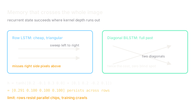
Two LSTM variants sweep the grid. The Row LSTM processes row by row with a $k \times 1$ state-to-state convolution: each row's states depend on the previous row's states, giving a triangular context that misses right-side pixels above. The Diagonal BiLSTM skews the image and sweeps diagonally in both directions, covering the full raster past at roughly twice the cost.

At each position the LSTM state feeds a $256$ -way softmax per channel, same output contract as PixelCNN. Residual connections between LSTM layers carry gradients through the depth.

Worked example

A $4$ -state toy Row LSTM at one position: input-to-state gives $[0.2, -0.1, 0.3, 0.0]$ , previous-row state contributes $[0.1, 0.2, -0.2, 0.1]$ , sums $[0.3, 0.1, 0.1, 0.1]$ , Tanh gives $[0.291, 0.100, 0.100, 0.100]$ . The state's largest component already encodes the strongest past signal, and that vector persists across the row while convolutions would have forgotten it within kernel range. Full Diagonal BiLSTM doubles this machinery for complete coverage.

Code

Row-state update in miniature, showing cross-row memory convolutions cannot carry.

1import numpy as np2
3
4def row_step(x_in: np.ndarray, h_prev_row: np.ndarray) -> np.ndarray:5    """One Row LSTM style update: fresh input plus previous row memory."""6    return np.tanh(x_in + h_prev_row)  # state persists across the row7
8
9print(np.round(row_step(np.array([0.2, -0.1, 0.3, 0.0]),10                        np.array([0.1, 0.2, -0.2, 0.1])), 3))  # -> [0.291 0.1 0.1 0.1]

Watch Out For

Training cost that dwarfs PixelCNN

Sequential row dependencies resist parallelisation far more than masked convolutions. PixelRNN trains several times slower than PixelCNN for modest likelihood gains, and the gap widens with image size.

Reserve PixelRNN for likelihood benchmarks where every nat counts. For generation quality per compute, later parallel architectures win.

Row LSTM blind spots mistaken for full context

The cheaper Row LSTM still misses right-side context above the current pixel. Teams deploy it expecting the paper's full-context numbers, which belong to the Diagonal BiLSTM, and wonder at the gap.

Name the variant in every result. Row and Diagonal BiLSTM are different models with different contexts and costs.

The Quick Version

PixelRNN sweeps LSTMs across the image so predictions see the full raster past.
Row LSTMs are cheap with triangular context; Diagonal BiLSTMs cover everything at double cost.
Our toy update yields state $[0.291, 0.100, 0.100, 0.100]$ persisting across rows.
Likelihood beats PixelCNN but training is far slower and harder to parallelise.
Name the variant always, and expect sampling to stay strictly sequential.