PixelCNN

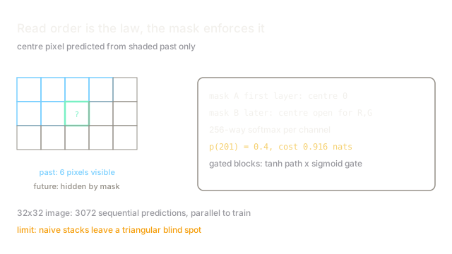
PixelCNN generates images one pixel at a time in reading order, using masked convolutions that let each pixel see only the pixels before it.

Masked convolutions hide future pixels so each prediction sees only the raster past

Why Does This Exist?

Likelihood was missing. GANs drew beautifully but assigned no probability to anything, leaving evaluation to arguments about samples. Density estimation on images needed a model with exact, tractable likelihood that still exploited spatial structure.

PixelCNN factorises the image into a product of conditionals in raster order and enforces the ordering architecturally: masked convolutions zero out every weight that could peek at the present or future. Training maximises exact log-likelihood with plain cross-entropy, and sampling walks the same order. The family overview is autoregressive image generation, and the recurrent sibling is PixelRNN.

Think of It Like This

A crossword writer who never looks ahead

A crossword setter fills the grid row by row, never glancing at unfilled squares. Each new letter must fit only the letters above and left, which constrains choices enough to keep words valid but forces awkward fills when an early guess paints the grid into a corner.

The mask is the rule against looking ahead. Generation is slow because letters commit one by one with no revision pass. It fails exactly where setters fail: globally planned structures, symmetry, long words that needed foresight the ordering forbids.

How It Actually Works

Order pixels $x_1, \dots, x_n$ row by row, and within a pixel order channels R then G then B. The model learns:

p(x) = \prod_i p(x_i \mid x_{<i}), \qquad p(x_{i,R}, x_{i,G}, x_{i,B}) = p(R) \, p(G \mid R) \, p(B \mid R, G)

Mask A on the first layer hides the centre pixel itself; Mask B on later layers allows seeing the centre's already-predicted channels. Each sub-pixel prediction is a $256$ -way softmax over colour values. Gated blocks, a Tanh filter path times a sigmoid gate path, carry the modelling capacity in deeper variants.

Worked example

Predicting a red value of $201$ with context giving it probability $0.4$ contributes $\log 0.4 = -0.916$ nats to the loss. A full $32 \times 32$ image holds $1{,}024$ pixels and $3{,}072$ channel predictions; at $2.0$ nats per channel the image costs $6{,}144$ nats, about $0.87$ bits per dimension. Sampling needs $3{,}072$ sequential network evaluations, which is why PixelCNN trains in parallel but generates one pixel at a time.

Code

Raster-scan loss over one row, showing the sequential factorization.

1import numpy as np2
3
4def raster_nll(probs: np.ndarray) -> float:5    """Negative log likelihood of the true values under predicted distributions."""6    return float(-np.log(probs).sum())7
8
9print(round(raster_nll(np.array([0.4, 0.7, 0.9])), 3))  # -> 1.378 nats

Watch Out For

Blind spots from naive masking

Stacked vertical-only masks ignore pixels to the right in rows above, a triangular blind spot covering half the context. Models train fine and underperform silently because context they should use never arrives.

Use two-stack (vertical plus horizontal) or gated horizontal stacks that cover the full raster past. Test receptive fields by gradient inspection, not by assumption.

Sampling too slow for interactive use

Parallel training hides the sequential bill until demo day: thousands of forward passes per image makes $64$ -pixel sampling take minutes. Users request bigger images and latency grows quadratically.

Cache intermediate activations across steps, distil into parallel samplers, or accept PixelCNN as a likelihood tool rather than a production generator.

The Quick Version

PixelCNN factorises images into raster-ordered pixel conditionals with masked convolutions.
Mask A hides the current pixel, Mask B admits already-predicted channels.
Each channel prediction is a $256$ -way classification with exact likelihood.
Our row example costs $1.378$ nats across three predictions.
Naive masks leave blind spots, and sequential sampling is inherently slow.