Pose Graph Optimization Backend

Poses are knots and measurements are elastic strings between them. Pose graph optimization relaxes the whole net until every string is as slack as possible.

Odometry edges chain poses while one loop edge pulls the ends together

Why Does This Exist?

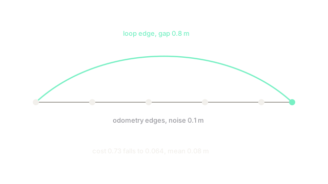
After loop closure fires, the system knows the ends should meet but the middle still holds the old drift. Pose graph optimization exists to distribute that correction: it adjusts every pose so odometry edges stay near their measured steps while the loop edge closes, instead of snapping one pose and kinking the path. It is the standard SLAM backend because it is far cheaper than full bundle adjustment over points.

This page covers the pose-only graph. Full camera-plus-point refinement is bundle adjustment; front-end motion is visual odometry.

Think of It Like This

A beaded necklace pulled shut

Beads on an elastic string form an almost-closed necklace with a gap between the ends. Clip the ends together and every bead shifts a little; none jumps across the table. The gap spreads evenly because every string segment pulls.

Poses are beads, odometry is the string, and the loop edge is the clip. The analogy stops at rotation: beads slide freely while 3D rotations need manifold updates, not plain averaging.

How It Actually Works

Nodes hold poses $T_i$ in $SE(3)$ ; edges hold measured relative motions $z_{ij}$ with information matrices $\Omega_{ij}$ encoding certainty. Error on an edge is $e_{ij} = z_{ij}^{-1} (T_i^{-1} T_j)$ mapped to a $6$ -vector via the logarithm map. The cost $C = \sum e_{ij}^T \Omega_{ij} e_{ij}$ is minimized with Gauss-Newton on the manifold, updating rotations through small axis-angle steps. Robust kernels such as Huber cap the influence of a wrong loop so one bad edge cannot fold the map.

Worked numbers

Ten poses chain with $0.1$ m noise each, ending $0.8$ m from the loop-verified reunion. The initial cost is dominated by the loop edge at $0.8^2 = 0.64$ . After five Gauss-Newton steps the gap spreads as $0.08$ m per edge, mean pose error $0.08$ m, and total cost falls to $10 \times 0.08^2 = 0.064$ , a tenfold drop.

Code

1def graph_cost(errors: list[float]) -> float:2    return sum(e * e for e in errors)  # unit information simplified3
4
5print(graph_cost([0.1] * 9 + [0.8]))  # -> 0.736print(graph_cost([0.08] * 10))  # -> 0.064

Watch Out For

Optimizing with a false loop edge

One wrong loop with high information bends corridors into pretzels while the cost looks improved. The symptom is a map that closes cleanly but disagrees with odometry everywhere. Verify loops geometrically and start new edges with a robust kernel, never full weight blindly.

The Quick Version

Pose graph nodes are poses; edges are measured relative motions.
The cost weights each edge error by its information matrix.
Loop edges close drift; odometry edges preserve local shape.
Manifold updates keep rotations valid during solving.
Robust kernels contain false loops instead of obeying them.
The backend spreads gap error evenly instead of kinking one pose.