ProGAN

ProGAN grows the generator and critic from thumbnails to megapixels, mastering each resolution before the next layer of detail is even added.

ProGAN masters 4 pixel thumbnails first, then fades in higher resolution layers one stage at a time

Why Does This Exist?

Jumping straight to $1024 \times 1024$ generation fails reliably. The critic instantly spots high-frequency flaws, gradients turn chaotic, and training collapses before the generator learns even coarse face layout. Resolution is the enemy of stability.

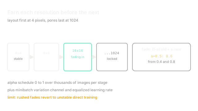
ProGAN sidesteps the fight by scheduling it. Both networks start at $4 \times 4$ , where the game is easy and layout is everything. Once thumbnails stabilise, a new layer fades in on each side and resolution doubles. By the time $1024$ pixels arrive, the generator already draws correct faces and only refines pores and hair. The style-based successor that builds on this schedule is StyleGAN, and the scale-driven cousin is BigGAN.

Think of It Like This

An art student who earns bigger canvases

A teacher starts a student on postage stamps: composition only, no detail possible. When stamps look right, the student graduates to postcards, then to posters, then to murals. Each new size arrives with the previous skills intact, so the mural has correct composition from day one and the student only practices fine brushwork.

Direct-to-mural students drown in detail before learning composition. The fade-in below is the graduation ceremony: the new canvas blends in gradually so skills transfer instead of resetting.

How It Actually Works

Training proceeds in stages $4 \to 8 \to \dots \to 1024$ , nine doublings. When a stage begins, the new high-resolution layers join through a fade-in: output is $(1 - \alpha) \times \text{upsampled old} + \alpha \times \text{new layers}$ , with $\alpha$ sliding $0 \to 1$ over thousands of images. At $\alpha = 0$ the network behaves exactly as the previous stage; at $\alpha = 1$ the new layers fully own the resolution.

Three stabilisers ride along. Minibatch standard deviation appends the batch's feature variation as a channel, so the critic notices collapsed batches directly. Equalised learning rate scales weights at runtime by $c/\sqrt{\text{fan-in}}$ , keeping update sizes uniform across layers. Pixelwise feature normalisation caps runaway magnitudes in the generator.

Worked example

Midway through the $16 \times 16$ fade with $\alpha = 0.5$ , a pixel's value is half the upsampled $8 \times 8$ output and half the new $16 \times 16$ layers. If the old path says $0.4$ and the new layers say $0.8$ , the output is $0.5 \times 0.4 + 0.5 \times 0.8 = 0.6$ . Early on the trusted old path dominates; late in the fade the new detail takes over without any sudden shock to the critic.

Code

Fade-in blending, the three lines that make growing painless.

1def fade_in(old: float, new: float, alpha: float) -> float:2    """Blend upsampled previous stage with fresh high-res layers."""3    return (1 - alpha) * old + alpha * new4
5
6print(fade_in(0.4, 0.8, 0.0))  # -> 0.4 previous stage only7print(round(fade_in(0.4, 0.8, 0.5), 2))  # -> 0.6 halfway through the fade8print(fade_in(0.4, 0.8, 1.0))  # -> 0.8 new layers fully own it

Watch Out For

Rushing the fade schedule

Double resolution every few thousand images and the new layers never integrate: $\alpha$ hits $1$ while the fresh convolutions still output noise, and the critic, suddenly facing garbage detail, destabilises the whole stack.

Hold each resolution until samples look clean at that size, typically hundreds of thousands of images per stage. The schedule is the method; hurrying it reverts to direct high-res training.

Forgetting minibatch statistics at sample time

Minibatch standard deviation needs a real batch to compute variation. Generate a single image and the statistic is degenerate, subtly shifting quality versus batch sampling.

Sample in batches even for demos, or accept the small single-sample shift. Never compare single-sample and batch-sample quality as if conditions matched.

The Quick Version

ProGAN grows both networks from $4 \times 4$ to $1024 \times 1024$ in nine doublings.
New layers fade in with $\alpha$ sliding $0 \to 1$ , blending old upsampled output with new detail.
At $\alpha = 0.5$ with paths $0.4$ and $0.8$ , the output is exactly $0.6$ .
Minibatch standard deviation, equalised learning rate, and pixel normalisation stabilise training.
Rushed schedules and single-sample generation are the two classic mistakes.