Sensor Fusion

Sensor fusion combines camera detail with lidar depth and radar velocity, so the car keeps working when any single sensor degrades.

Camera, lidar, and radar contribute complementary evidence that fuses into one track

Why Does This Exist?

Cameras read texture but guess depth. Lidar measures depth but thins with range and fails in heavy spray. Radar reports velocity directly but localizes poorly. Any single sensor has a weather or range where it quits. Sensor fusion exists to arrange complementary quits: when glare blinds the camera, lidar holds shape; when spray scatters lidar, radar holds speed. The fused track outlives each sensor alone.

The full BEV system is BEV perception and sensor fusion; this page owns the fusion choice itself.

Think of It Like This

Three witnesses with different strengths

One witness remembers faces, one paces distances exactly, one hears how fast things move. Alone each misleads sometimes, together they convict. The car treats cameras, lidar, and radar the same way, weighting each by conditions. The analogy stops at testimony: sensors need microsecond timing and millimeter calibration to agree at all.

How It Actually Works

Early fusion concatenates raw or voxel features before detection. Late fusion runs per-sensor detectors then associates tracks. Middle fusion shares BEV features, the current favored point. Each observation carries a covariance $R$ stating its noise. Fusion weights follow inverse noise: a camera box with high blur gets low weight while radar velocity keeps full weight. Time sync aligns timestamps; extrinsic calibration aligns frames.

Worked example

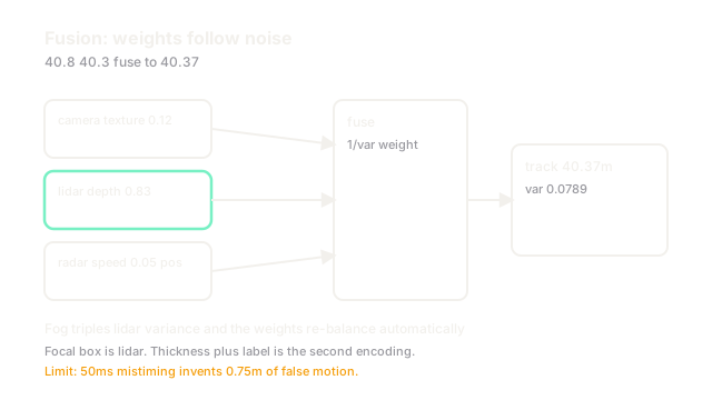
A car at 40 m is seen by camera with lateral noise 0.8 m, by lidar with 0.3 m, by radar with 1.2 m lateral but 0.2 m per s velocity noise. Inverse-variance weights for position are about 0.12, 0.83, and 0.05, so lidar dominates position while radar dominates speed. In fog the lidar variance triples and camera weight rises relatively, which the filter does automatically when covariances reflect conditions.

Code

This snippet fuses two position estimates by inverse variance.

1import numpy as np2
3
4def fuse(xs: list[float], vars_: list[float]) -> tuple[float, float]:5    w = np.array([1.0 / v for v in vars_])6    x = float((w * np.array(xs)).sum() / w.sum())7    return round(x, 3), round(float(1.0 / w.sum()), 4)8
9
10print(fuse([40.8, 40.3], [0.64, 0.09]))  # -> (40.37, 0.0789)

Lidar at variance 0.09 pulls the 40.37 estimate toward itself and shrinks uncertainty below either input.

Watch Out For

Silent mistiming that bends velocity

A 50 ms camera-lidar offset at 15 m per s shifts associations by 0.75 m, so the filter invents lateral velocity to explain the gap. The symptom is oscillating headings on straight roads. Timestamp at the sensor, compensate for exposure and sweep time, and monitor delay residuals rather than assuming zero.

The Quick Version

Cameras give texture, lidar gives depth, radar gives velocity.
Fusion places them in one frame at one time before deciding.
Weights follow noise, so the best sensor per condition leads.
Calibration and sync failures look like perception failures.
Design for complementary degradation, not average accuracy.