Spatio-Temporal Transformers

Video is space plus time, and attention can span both — at quadratic cost. Spatio-temporal transformers factor the attention so frames talk within and across time affordably.

Divided attention prices 0.32 million comparisons against 2.46 million joint, nearly 8 times cheaper

Why Does This Exist?

3-D convolutions see locally in time; full space-time attention sees everything at impossible cost. A modest clip ( $8$ frames, $196$ patches each) holds $1{,}568$ tokens, and joint attention prices $1{,}568^2 \approx 2.5$ million comparisons per head per layer — before going long. Video needed attention's range without its bill.

Spatio-temporal transformers factor the operation: temporal attention per spatial position, then spatial attention per frame (TimeSformer's divided scheme), or tubelet embeddings plus factorized encoders (ViViT). Cross-frame reasoning survives at a fraction of the price. The pretrained users are video foundation models; the live users are streaming models.

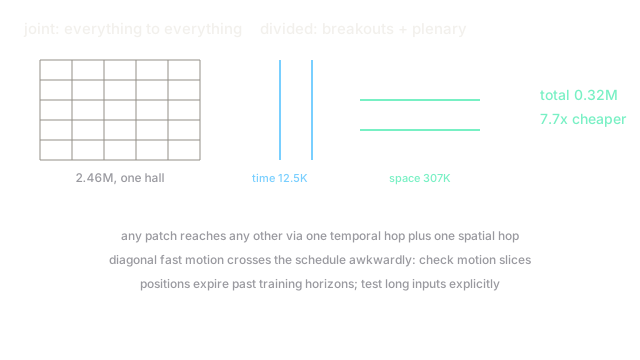
The one idea you need first. Divided attention runs two cheaper passes instead of one giant one: each patch first attends across time at its own position ( $T \times T$ per patch), then across space within its frame ( $S \times S$ per frame). Information still flows from any patch to any other — via a temporal hop plus a spatial hop — while the comparison count drops roughly eightfold.

Think of It Like This

Breakout rooms, then plenary

A $1{,}500$ -person conference cannot hold one conversation: all-to-all talk is noise at quadratic cost. Organizers split time into breakout rooms (local groups converse cheaply), then plenary (each room reports, everyone syncs). Every idea still reaches every ear — via room plus stage instead of direct shout.

Divided attention is that schedule. Temporal attention is the breakout (each position's timeline converses); spatial attention is the plenary (each frame syncs). Joint attention insists on the single giant hall and pays the noise bill; factorization keeps the reach and drops the price.

How It Actually Works

Tokenize frames into patches (or spacetime tubelets spanning $2$ frames to halve counts). Alternate temporal and spatial blocks: temporal first lets motion features form before spatial mixing (the TimeSformer order that ablates best), with learned space-time positional encodings keeping coordinates straight. Classification pools a class token or averages; dense tasks keep full resolution. Long-video variants add windowed, axial, or memory-compressed attention on top of the divided base.

Complexity per layer drops from $O((TS)^2)$ to $O(T^2S + TS^2)$ — same reach, scheduled sensibly.

Worked example

$T = 8$ frames, $S = 196$ patches: $1{,}568$ tokens.

Joint: $1{,}568^2 = 2{,}458{,}624 \approx 2.46$ M comparisons.
Divided temporal: per patch $8^2 = 64$ ; over $196$ patches $64 \times 196 = 12{,}544$ .
Divided spatial: per frame $196^2 = 38{,}416$ ; over $8$ frames $38{,}416 \times 8 = 307{,}328$ .
Total: $12{,}544 + 307{,}328 = 319{,}872 \approx 0.32$ M. Ratio: $2{,}458{,}624 / 319{,}872 \approx 7.7$ .

Nearly eightfold cheaper per layer, every layer, compounding through depth — the margin that makes video transformers trainable.

Code

The point of this snippet is the bill: joint versus divided counts reproduce the $7.7\times$ margin.

1def attention_bills(frames: int, patches: int) -> tuple:2    joint = (frames * patches) ** 23    divided = frames**2 * patches + patches**2 * frames4    return joint, divided5
6
7joint, divided = attention_bills(8, 196)8print(joint, divided)  # -> (2458624, 319872)9print(round(joint / divided, 1))  # -> 7.7

Watch Out For

Diagonal motion the factorization blurs

Divided passes mix time-then-space, so fine diagonal trajectories (motion plus position changing together) cross the factorization awkwardly — each pass sees half the pattern. Small fast objects suffer most, exactly where tracking needs them sharp.

Check motion-heavy slices when choosing factorization; tubelet embeddings (spanning time at tokenization) recover part of the diagonal. Joint attention on short clips remains the accuracy reference.

Positions that expire past the horizon

Learned space-time encodings memorize training lengths; feeding $4\times$ longer videos at inference scrambles coordinates the model never learned. Performance cliffs at the pretraining horizon, silently.

Use relative or extrapolatable encodings for long targets, and test past-horizon explicitly before claiming length generalization. The cliff sits exactly where demos stop measuring.

The Quick Version

Spatio-temporal transformers factor attention into temporal-then-spatial passes at $O(T^2S + TS^2)$ .
The worked fixture prices divided at $0.32$ M versus joint $2.46$ M: $7.7\times$ cheaper per layer.
Reach survives via two-hop paths (temporal plus spatial) instead of direct all-to-all.
Diagonal fast motion crosses factorizations awkwardly; verify on motion-heavy slices.
Learned positions expire past training horizons, so test long inputs explicitly.