Spherical CNNs

Panoramas and omnidirectional cameras see in spheres, not rectangles. Spherical CNNs convolve directly on the sphere, so a rotated camera still sees the same features in the same way.

Flat projection stretches polar regions nearly sixfold while spherical convolution keeps one uniform kernel everywhere

Why Does This Exist?

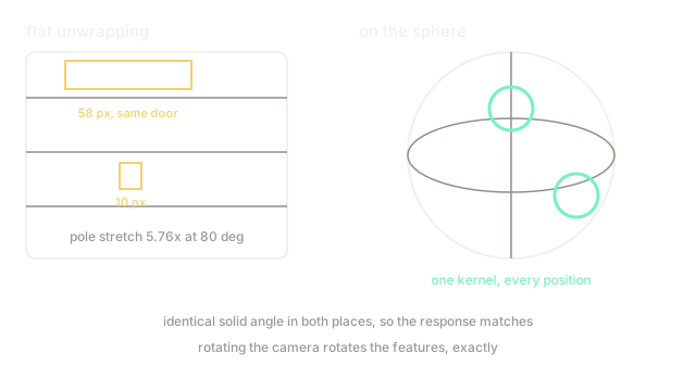
A $360$ -degree camera unwrapped into a rectangle lies about its poles. Equirectangular projection stretches high latitudes enormously, so a doorway near the zenith smears across dozens of pixels while the same doorway at the equator stays compact. A flat CNN meets two different patterns for one object and learns both, wasting capacity on an artifact of the unwrapping.

Spherical CNNs skip the unwrapping. Signals live on the sphere $S^2$ , filters correlate over the rotation group $SO(3)$ , and rotating the camera rotates the features exactly. Drones, robots, and AR headsets with omnidirectional sensors get rotation-proof perception. The flat-rotation sibling is steerable networks; the principle is geometric deep learning.

The one idea you need first. Correlation on the rotation group replaces sliding a kernel over $(x, y)$ with integrating over all 3D rotations. The output lives on $SO(3)$ — one response per orientation — and rotating the input permutes those responses the way shifting an image shifts CNN feature maps. Fast algorithms via spherical harmonics (the sphere's Fourier basis) keep this tractable.

Think of It Like This

A globe versus a Mercator wall map

Greenland on a Mercator map looks bigger than Africa; on a globe it is a small island. The wall map stretches the poles to fit a rectangle, and navigators who forget the stretching misjudge every northern route. The globe distorts nothing because it never pretends the Earth is flat.

Flat CNNs on panoramas read the wall map: polar regions arrive pre-stretched, and the network must learn the stretching as if it were object shape. Spherical CNNs read the globe. One kernel means one pattern everywhere, and the poles stop being special cases that eat capacity.

The analogy stops at cost: globes are harder to manufacture, and spherical correlation costs more compute than flat convolution for the same resolution.

How It Actually Works

The first layer correlates the spherical signal with a learnable filter over $SO(3)$ , producing one feature per rotation. Deeper layers convolve rotation-group features with rotation-group filters, reusing weights across orientations. Spherical harmonics convert both signal and filter into frequency coefficients where rotation becomes a clean matrix multiplication, enabling a generalized FFT instead of brute-force integration over angles.

Equivariance is exact in the continuous setting and approximate after discretization onto a sampling grid (equiangular or HEALPix). Final invariant predictions come from pooling over $SO(3)$ ; pose estimation keeps the group dimension.

Worked example

Quantify the distortion a spherical CNN avoids. Equirectangular projection stretches a pixel at latitude $\phi$ by $1 / \cos\phi$ horizontally. At the equator ( $\phi = 0$ ), $\cos 0 = 1$ , stretch $1.0$ : no distortion. At $\phi = 80$ degrees near the pole, $\cos 80^\circ \approx 0.1736$ , so the stretch is $1 / 0.1736 \approx 5.76$ .

A doorway $10$ pixels wide at the equator arrives $58$ pixels wide near the pole — nearly sixfold wider for the identical object. A flat kernel sized for one fails the other; a spherical kernel meets the same solid angle in both places and responds identically.

Code

The point of this snippet is the stretch factor: two lines show why polar unwrapping breaks flat kernels while spherical ones are unaffected.

1import math2
3
4def equirectangular_stretch(lat_deg: float) -> float:5    return 1.0 / math.cos(math.radians(lat_deg))  # horizontal stretch factor6
7
8print(round(equirectangular_stretch(0), 2))  # -> 1.09print(round(equirectangular_stretch(80), 2))  # -> 5.7610print(round(10 * equirectangular_stretch(80)))  # -> 58

Ten equatorial pixels become about $58$ near the pole: the number a flat network must absorb and a spherical network never sees.

Watch Out For

Bandwidth cost grows faster than resolution

Spherical harmonic transforms scale steeply with the bandwidth $B$ (roughly $O(B^3)$ ), so doubling angular resolution multiplies compute about eightfold. Teams porting flat architectures layer-for-layer hit a wall around moderate resolutions.

Design at low bandwidth first and verify the task is solvable there; add resolution only with measurements. Most orientation-sensitive tasks (pose, layout) resolve well before the compute budget runs out.

Sampling grids are not rotation-proof

Exact equivariance lives in the continuous math. Real implementations sample the sphere, and rotating the input between grid points introduces aliasing the theory does not cover. Scores on arbitrary rotations sag slightly versus on-grid ones.

Use uniform grids (HEALPix over naive equiangular), and validate with continuous camera rotations rather than the sampled set. The gap is small but real, and it concentrates exactly where the guarantee was supposed to apply.

The Quick Version

Spherical CNNs correlate over the rotation group $SO(3)$ instead of sliding kernels on an unwrapped rectangle.
The worked fixture shows polar unwrapping stretches patterns $5.76$ -fold at $80$ degrees latitude.
Rotating the camera rotates spherical features exactly, replacing pole-specific learning with one kernel.
Cost grows steeply with angular bandwidth, so design coarse first and measure before refining.
Discrete sampling grids reintroduce small rotation gaps through aliasing, so validate continuously.