Geometric and Equivariant Deep Learning

Images rotate, cameras move in 3D, and data lives on surfaces rather than flat grids. Geometric deep learning builds networks that respect those symmetries instead of relearning them from extra data.

One equivariance rule covers vision symmetries: transforming the input transforms the features the same way, across grids, spheres, and graphs

Why Does This Exist?

Convolutional networks won vision partly because of one symmetry: shift an image and the feature maps shift with it. Nobody augments with every possible translation, because translation handling is built in. Every other symmetry — rotation, reflection, 3D pose, permutation of points — was left for brute-force augmentation: copy the data four ways, train four times as long, and hope.

Geometric deep learning generalizes the trick. Name the symmetry as a group, then constrain the layers so features transform predictably under it. The payoff is data efficiency where augmentation is expensive (3D rotations, spherical cameras) and guarantees where augmentation gives none. This page states the shared principle and maps the family: group equivariant CNNs, steerable networks, spherical CNNs, and graph networks for vision.

The one idea you need first. A group is a set of transformations with clean algebra: rotations by multiples of $90$ degrees compose, undo, and include doing nothing. Equivariance means the network commutes with the transformation: transform the input, and the features transform the same way. In symbols, $f(g \cdot x) = g \cdot f(x)$ . Invariance is the special case where the output does not move at all, so classification usually ends invariant while intermediate features stay equivariant.

Think of It Like This

A compass that works however you hold the map

A cheap compass rose printed on a paper map only reads correctly when the map faces north. Turn the map and every reading is wrong until you redo the math. A magnetic compass works however you hold it: the needle keeps pointing north and your reading transforms along with your grip.

Standard CNNs are the printed rose: reliable for shifts, lost on rotations unless retrained at every angle. Equivariant networks are the magnetic needle. The symmetry is inside the mechanism, so turning the input turns the features by the same amount with no relearning, and the final decision can read the needle from any orientation.

The analogy stops at construction: nobody hand-builds the needle. The constraint is written into the layer algebra, and training fills in the rest.

How It Actually Works

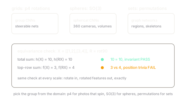
The blueprint has three steps. First, identify the symmetry group $G$ of the domain: translations plus $90$ -degree rotations ( $p4$ ) for upright photos, full 3D rotations ( $SO(3)$ ) for volumes and panoramas, permutations for point sets and graphs. Second, pick how features transform: scalars stay put, vectors rotate, orientation channels permute. Third, constrain each layer to commute with $G$ , usually by sharing weights over transformed copies of the filter.

A tiny numeric check shows what commuting means. Take $X = [[1, 2], [3, 4]]$ and a $90$ -degree clockwise rotation $R$ , giving $RX = [[3, 1], [4, 2]]$ . Let $f$ sum the top row: $f(X) = 1 + 2 = 3$ , while $f(RX) = 3 + 1 = 4$ . Rotating a scalar output leaves $3$ unchanged, and $3 \neq 4$ , so this $f$ is not equivariant — it reads position-dependent trivia. Now let $g$ sum everything: $g(X) = 10$ and $g(RX) = 10$ . Equal, as invariance demands. Real equivariant layers pass the first style of test with feature-valued outputs: rotate in, rotated features out, exactly.

Worked example

Test a candidate layer the way you would test code. Input $X = [[1, 2], [3, 4]]$ , rotation $R$ as above, candidate $h$ = "sum of all entries":

Compute $h(X) = 1 + 2 + 3 + 4 = 10$ .
Rotate first: $RX = [[3, 1], [4, 2]]$ , then $h(RX) = 3 + 1 + 4 + 2 = 10$ .
Compare under the output's transformation (scalars do not move): $10 = 10$ . Pass — invariant.

Repeat with $f$ = "top row sum": $f(X) = 3$ versus $f(RX) = 4$ . Fail — position-sensitive. Every equivariant architecture in this family is this check, lifted from $2 \times 2$ toys to whole layer stacks.

Code

The point of this snippet is the equivariance test itself: implement it once and run every candidate layer through it before trusting its symmetry claims.

1from typing import Callable2
3
4def rot90_clockwise(m: list) -> list:5    return [list(row) for row in zip(*m[::-1])]  # transpose the reversed rows6
7
8def is_invariant(fn: Callable, x: list) -> bool:9    return fn(rot90_clockwise(x)) == fn(x)  # scalars must not move10
11
12X = [[1, 2], [3, 4]]13print(rot90_clockwise(X))  # -> [[3, 1], [4, 2]]14print(is_invariant(lambda m: sum(sum(row) for row in m), X))  # -> True15print(is_invariant(lambda m: sum(m[0]), X))  # -> False

Watch Out For

Assuming a symmetry the data does not have

Equivariance to full rotation on upright photos (digits 6 versus 9, faces, text) actively destroys information: the network is forced to treat orientations as equivalent when the task needs them distinguished. Accuracy falls and no amount of tuning recovers it, because the constraint forbids the solution.

Match the group to the domain. Use rotation equivariance for aerial imagery, microscopy, and molecules; keep upright-photo models translation-only. The symmetry is a claim about the world, and a wrong claim is worse than no claim.

Discrete groups leave gaps between samples

A $p4$ network handles $0$ , $90$ , $180$ , and $270$ degrees exactly and improvises at $45$ degrees. Test accuracy often dips midway between the group's angles, which surprises teams who read "rotation equivariant" as "rotation proof".

Probe the gaps deliberately: sweep rotation continuously on validation and plot the curve. If the dips matter, move to steerable networks for continuous coverage rather than stacking more augmentation on a discrete group.

The Quick Version

Geometric deep learning constrains layers to commute with a symmetry group: $f(g \cdot x) = g \cdot f(x)$ .
The worked fixture shows a total sum passing the rotation test ( $10 = 10$ ) while a top-row sum fails ( $3 \neq 4$ ).
One blueprint covers grids, spheres, and graphs; only the group and the feature types change.
Pick the group from the domain: wrong symmetries destroy orientation information the task needs.
Discrete groups leave gaps between sampled angles, so sweep rotations continuously when validating.