Thresholding-Based Segmentation

Pick one brightness cutoff and every pixel brighter than it becomes foreground while everything darker becomes background. Simple, instant, and surprisingly far-reaching.

Otsu's method picks the cutoff that maximizes between-class variance, splitting the histogram at the valley between its two peaks.

Why Does This Exist?

Plenty of vision jobs end in a yes-or-no question per pixel: is this ink or paper, cell or slide, coin or table? Classical segmentation surveys the whole family, but thresholding deserves its own page because it answers that question with a single comparison, no training data, and microseconds of compute. Scanned documents, microscopy slides, and industrial inspection lines still binarize this way before anything fancier runs.

You need one prerequisite idea first: brightness lives in a single channel, so color images get reduced to luminance before any of this applies. The details are in color spaces. This page covers the global cutoff rule, Otsu's automatic choice, adaptive windows, and multilevel splits. Connected regions and touching objects belong to region growing and watershed segmentation instead.

Think of It Like This

Sorting gravel with a sieve

Pour mixed gravel over a sieve and every stone smaller than the mesh falls through while everything larger stays on top. The mesh size is the threshold $T$ : one number decides every stone, you never inspect a stone twice, and the whole pile is sorted in one pass.

It stops holding where sieves always stop: size is the only thing a sieve can see. A small gold nugget falls through with the sand, the same way a dark foreground pixel on a shadowed background gets labeled background. One property, one decision, no second chances.

How It Actually Works

The global cutoff rule

A grayscale image $I(x, y)$ becomes a binary mask $g(x, y)$ through one comparison against a threshold $T$ :

$g(x, y) = 1$ when $I(x, y) > T$ , else $0$ .

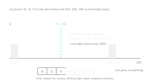
Take six pixels with values $[10, 12, 11, 200, 205, 198]$ . With $T = 100$ , the first three fall below and the last three clear it, giving three background pixels with mean $11$ and three foreground pixels with mean $201$ . Every pixel is classified, nothing is learned, and the cost is one pass over the image.

Otsu's automatic threshold

Hand-picking $T$ fails the moment lighting shifts, so Otsu's method (1979) picks it from the histogram. For each candidate $T$ it splits pixels into two classes with weights $w_0, w_1$ and means $\mu_0, \mu_1$ , then scores the split with the between-class variance $\sigma_B^2 = w_0 w_1 (\mu_0 - \mu_1)^2$ . The $T$ with the largest score wins.

On the six pixels above, splitting between $12$ and $198$ gives $w_0 = w_1 = 0.5$ , means $11$ and $201$ , and $\sigma_B^2 = 0.25 \times 190^2 = 9025$ . The only other plausible split, $\{10, 11\}$ against the rest, scores $w_0 w_1 (\mu_0 - \mu_1)^2 = (1/3)(2/3)(143.25)^2 \approx 4560$ . Otsu picks the $9025$ split, exactly the gap a human eye sees. The method assumes a bimodal histogram, and that assumption is also its limit.

Adaptive windows and multilevel splits

When illumination drifts across the frame, one global $T$ cannot work: the lit side washes out or the shaded side goes black. Adaptive thresholding computes a separate $T$ per pixel from its neighborhood mean or Gaussian-weighted average, minus a small constant. Multilevel thresholding goes the other direction, using two cutoffs to split pixels into three bands, which suits images with a mid-tone class such as gray matter between white matter and background in brain scans.

Code

Pure-Python Otsu on the six-pixel fixture, checking every midpoint split:

1pixels = [10, 12, 11, 200, 205, 198]2
3def score(split):4    bg = [p for p in pixels if p <= split]5    fg = [p for p in pixels if p > split]6    if not bg or not fg:7        return 0.08    w0, w1 = len(bg) / len(pixels), len(fg) / len(pixels)9    m0 = sum(bg) / len(bg)10    m1 = sum(fg) / len(fg)11    return w0 * w1 * (m0 - m1) ** 212
13cands = [(a + b) / 2 for a, b in zip(sorted(pixels), sorted(pixels)[1:])]14best = max(cands, key=score)15print(f"best split {best}, variance {score(best):.0f}")16# -> best split 105.0, variance 9025

The winning split sits at $105$ , midway between $12$ and $198$ , with variance $9025$ , matching the hand computation above.

Watch Out For

Using one global threshold under uneven light

Symptom: half the document binarizes perfectly and the other half turns solid black or white, with the failure following the shadow line. A single $T$ cannot serve two illumination zones. Fix it with adaptive thresholding or by estimating the background (morphological closing with a large structuring element) and subtracting it before Otsu.

Trusting Otsu on a non-bimodal histogram

Otsu always returns a number, even on a flat or single-peak histogram where no good split exists. Symptom: the mask looks arbitrary and tiny lighting changes swing the threshold wildly. Plot the histogram first. If you do not see two humps, thresholding is the wrong tool and you want region or edge-based methods instead.

The Quick Version

Thresholding labels each pixel foreground or background with one comparison against a cutoff $T$ .
Otsu's method finds $T$ automatically by maximizing the between-class variance $w_0 w_1 (\mu_0 - \mu_1)^2$ .
Adaptive thresholding computes a local $T$ per pixel, which survives uneven illumination that kills global cutoffs.
Multilevel thresholding uses two cutoffs for images with a genuine mid-tone class.
It needs no training data but assumes brightness alone separates the classes, so camouflaged objects defeat it completely.