Transformer-based Detectors

DETR replaces hand-crafted anchor boxes and NMS with a transformer encoder-decoder and bipartite Hungarian matching for true end-to-end detection.

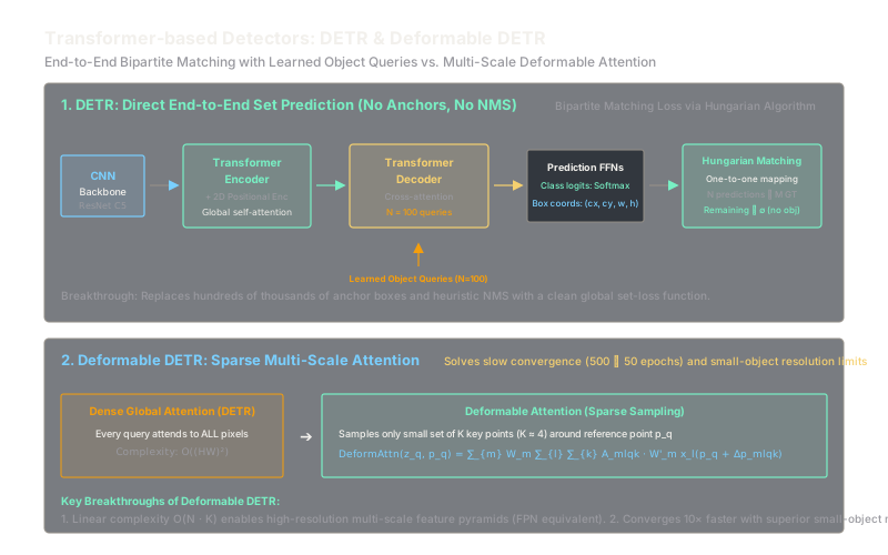
DETR transformer architecture with learned object queries and Hungarian matching alongside Deformable DETR multi-scale sparse sampling.

Why Does This Exist?

Traditional object detectors such as Faster R-CNN and YOLO rely heavily on hand-crafted engineering heuristics:

Anchor box design: Thousands of predefined bounding boxes with manually tuned spatial scales and aspect ratios that vary wildly between datasets.
Rule-based label assignment: Complex IoU overlap thresholds (e.g., $\text{IoU} > 0.7$ foreground, $\text{IoU} < 0.3$ background) to match predictions to ground truth.
Non-Maximum Suppression (NMS): Greedy post-processing steps that cannot be differentiated end-to-end and frequently fail in dense, crowded scenes.

These hand-tuned components made detection pipelines difficult to optimize and deploy cleanly across edge devices.

DETR (DEtection TRansformer, Carion et al., 2020) fundamentally re-imagined object detection as a direct set prediction problem. By pairing a standard CNN backbone with a transformer encoder-decoder and an end-to-end bipartite matching loss, DETR eliminated anchor boxes, rule-based assignment, and NMS entirely.

However, original DETR suffered from two major limitations: very slow training convergence (requiring 500 epochs to match Faster R-CNN) and weak performance on small objects due to quadratic computational complexity $O((HW)^2)$ that prevented processing high-resolution feature maps. Deformable DETR (Zhu et al., 2020) resolved both bottlenecks using sparse, multi-scale deformable attention modules that sample only a few key reference points, cutting training time by $10\times$ (converging in 50 epochs).

Think of It Like This

A lottery ticket grid vs. an elite auction with numbered paddles

Imagine locating valuable antiques hidden throughout an estate sale.

Traditional anchor-based detectors (like Faster R-CNN or YOLO) carpet the entire house with 100,000 pre-printed lottery tickets: one for every square foot, every doorway, every tabletop. Many tickets will accidentally overlap the same antique chair. Afterwards, a cleaning crew has to rummage through the pile (NMS) to throw out redundant duplicates.

DETR operates like a private auction room with exactly $N=100$ numbered bidder paddles (the Object Queries). The transformer encoder reads the entire room inventory at once, taking in global context. Then, all 100 bidders raise their paddles simultaneously. Bidder 1 bids on the antique clock by the mantle; Bidder 2 bids on the oil painting above the sofa; Bidders 3 through 100 conclude there are no other antiques in the room and bid on "empty background" ( $\varnothing$ ).

An automated auction arbiter (the Hungarian matching algorithm) guarantees that each physical antique is awarded to at most one bidder. Because each antique has exactly one winner, there are no duplicates to delete and no NMS is needed.

How It Actually Works

The DETR Set Prediction Pipeline

Backbone Feature Extraction: A CNN backbone (e.g., ResNet-50) processes an input image $x_{\text{img}} \in \mathbb{R}^{3 \times H \times W}$ into a low-resolution feature map $f \in \mathbb{R}^{C \times \frac{H}{32} \times \frac{W}{32}}$ . A $1 \times 1$ convolution reduces channels from $C=2048$ to $d=256$ .
Transformer Encoder: The spatial dimensions are flattened into a 1D sequence of length $L = \frac{HW}{1024}$ . Fixed 2D spatial sine-cosine positional encodings are added to each token. Standard multi-head self-attention models global pairwise spatial relationships across the entire image.
Transformer Decoder & Object Queries: The decoder takes $N$ learnable positional embeddings called Object Queries (typically $N = 100$ ). Through alternating self-attention and cross-attention over the encoder's memory, the queries iteratively interact and localize distinct physical objects.
Prediction Feedforward Networks (FFNs): Each of the $N$ $N$ output embeddings passes through independent 3-layer MLPs:
- Linear classification head: outputs class probabilities over $K + 1$ classes (including the null class $\varnothing$ ).
- Bounding box regression head: outputs normalized box coordinates $\hat{b} = (\hat{c}_x, \hat{c}_y, \hat{w}, \hat{h}) \in [0, 1]^4$ .

Hungarian Bipartite Matching Loss

Let $y = \{y_i\}_{i=1}^M$ be the ground-truth set of objects, padded with null tokens $\varnothing$ up to size $N$ . We search for a permutation of $N$ elements $\sigma \in \mathfrak{S}_N$ with the lowest matching cost:

\hat{\sigma} = \arg\min_{\sigma \in \mathfrak{S}_N} \sum_{i=1}^{N} \mathcal{L}_{\text{match}}\left(y_i, \hat{y}_{\sigma(i)}\right)

The pairwise matching cost between ground truth $y_i = (c_i, b_i)$ and prediction $\hat{y}_\sigma$ with predicted class probability $\hat{p}_{\sigma(i)}(c_i)$ and box $\hat{b}_{\sigma(i)}$ is:

\mathcal{L}_{\text{match}}(y_i, \hat{y}_{\sigma(i)}) = - \mathbf{1}_{\{c_i \neq \varnothing\}} \hat{p}_{\sigma(i)}(c_i) + \mathbf{1}_{\{c_i \neq \varnothing\}} \mathcal{L}_{\text{box}}(b_i, \hat{b}_{\sigma(i)})

where the bounding box loss combines $L_1$ loss and Generalized IoU (GIoU) loss:

\mathcal{L}_{\text{box}}(b_i, \hat{b}_{\sigma(i)}) = \lambda_{\text{L1}} \| b_i - \hat{b}_{\sigma(i)} \|_1 + \lambda_{\text{giou}} \mathcal{L}_{\text{giou}}(b_i, \hat{b}_{\sigma(i)})

The optimal one-to-one assignment $\hat{\sigma}$ is solved efficiently in $O(N^3)$ time using the Hungarian algorithm. Once matched, the network computes standard cross-entropy and box regression losses over the assigned pairs.

Deformable DETR: Multi-Scale Deformable Attention

Standard transformer self-attention over an image feature map calculates $H \times W$ dot products for every single query point, resulting in prohibitive $O((HW)^2)$ complexity.

Deformable DETR replaces full attention with multi-scale deformable attention. Given an input feature map $x$ and a 2D reference point $p_q$ , the deformable attention module queries only a small fixed set of $K$ sampling points (typically $K = 4$ ) per attention head across $L$ feature levels:

\text{DeformAttn}\left(z_q, p_q, \{x^l\}\right) = \sum_{m=1}^{M} W_m \sum_{l=1}^{L} \sum_{k=1}^{K} A_{mlqk} \cdot W'_m x^l\left(\phi_l(p_q) + \Delta p_{mlqk}\right)

where:

$m$ indexes the attention head, $l$ indexes the feature level (FPN scale), and $k$ indexes the sampled key point.
$\Delta p_{mlqk}$ is a continuous 2D sampling offset predicted by a linear projection of the query embedding $z_q$ .
$A_{mlqk} \in [0, 1]$ is a normalized attention weight ( $\sum_{l, k} A_{mlqk} = 1$ ).
Bilinear interpolation evaluates $x^l$ at non-integer coordinates $\phi_l(p_q) + \Delta p_{mlqk}$ .

Because $K$ is small and fixed, complexity drops to $O(N_{\text{query}} \cdot C + N_{\text{key}} \cdot C)$ , making multi-scale processing fast and practical.

Worked Example

Consider matching $N = 3$ predictions against $M = 2$ ground-truth objects (with 1 null token $\varnothing$ ).

Ground-truth objects:

$y_1$ : Cat at $b_1 = [0.2, 0.2, 0.4, 0.4]$
$y_2$ : Dog at $b_2 = [0.7, 0.7, 0.3, 0.3]$
$y_3$ : Null token $\varnothing$

Predictions:

$\hat{y}_1$ : Predicts Cat with $p=0.85$ at $\hat{b}_1 = [0.22, 0.19, 0.38, 0.41]$
$\hat{y}_2$ : Predicts Dog with $p=0.80$ at $\hat{b}_2 = [0.68, 0.71, 0.31, 0.29]$
$\hat{y}_3$ : Predicts Dog with $p=0.20$ at $\hat{b}_3 = [0.10, 0.10, 0.20, 0.20]$

Let simplified cost be: $\text{Cost}(y_i, \hat{y}_j) = -p_j(c_i) + \| b_i - \hat{b}_j \|_1$ (for $c_i \neq \varnothing$ , 0 otherwise):

For $y_1$ $y_{1}$ (Cat):
- With $\hat{y}_1$ : $-0.85 + (\left|0.2-0.22\right| + \left|0.2-0.19\right| + \left|0.4-0.38\right| + \left|0.4-0.41\right|) = -0.85 + (0.02 + 0.01 + 0.02 + 0.01) = -0.85 + 0.06 = -0.79$
- With $\hat{y}_2$ : $-0.05 + \|b_1 - \hat{b}_2\|_1 \approx -0.05 + 1.88 = +1.83$
- With $\hat{y}_3$ : $-0.10 + \|b_1 - \hat{b}_3\|_1 \approx -0.10 + 0.60 = +0.50$
For $y_2$ $y_{2}$ (Dog):
- With $\hat{y}_1$ : $-0.05 + 1.88 = +1.83$
- With $\hat{y}_2$ : $-0.80 + (\left|0.7-0.68\right| + \left|0.7-0.71\right| + \left|0.3-0.31\right| + \left|0.3-0.29\right|) = -0.80 + 0.05 = -0.75$
- With $\hat{y}_3$ : $-0.20 + 2.40 = +2.20$

Cost matrix:

\mathbf{C} = \begin{bmatrix} -0.79 & +1.83 & +0.50 \\ +1.83 & -0.75 & +2.20 \\ 0 & 0 & 0 \end{bmatrix}

The Hungarian algorithm selects the optimal assignment: $\sigma = (1 \to \hat{y}_1, 2 \to \hat{y}_2, 3 \to \hat{y}_3)$ with total cost $-0.79 - 0.75 + 0 = -1.54$ . Bipartite matching cleanly associates prediction 1 with the Cat, prediction 2 with the Dog, and leaves prediction 3 to be penalized as background!

Code

1import torch2from scipy.optimize import linear_sum_assignment3
4def hungarian_matching(5    pred_logits: torch.Tensor,6    pred_boxes: torch.Tensor,7    gt_labels: torch.Tensor,8    gt_boxes: torch.Tensor,9    cost_class: float = 1.0,10    cost_bbox: float = 5.011) -> list[tuple[int, int]]:12    """Solve optimal bipartite matching between DETR predictions and ground truth.13    pred_logits: shape (N, num_classes)14    pred_boxes:  shape (N, 4) in (cx, cy, w, h)15    gt_labels:   shape (M,)16    gt_boxes:    shape (M, 4)17    """18    n = pred_logits.shape[0]19    m = gt_labels.shape[0]20
21    # Compute softmax class probabilities22    out_prob = pred_logits.softmax(-1)23    24    # Classification cost: -prob for ground truth class25    cost_class_matrix = -out_prob[:, gt_labels]  # (N, M)26    27    # L1 Bounding box cost28    cost_bbox_matrix = torch.cdist(pred_boxes, gt_boxes, p=1)  # (N, M)29    30    # Combined cost matrix (N, M)31    cost_matrix = cost_class * cost_class_matrix + cost_bbox * cost_bbox_matrix32    cost_matrix = cost_matrix.detach().cpu().numpy()33    34    # Solve Hungarian assignment35    pred_ind, gt_ind = linear_sum_assignment(cost_matrix)36    return list(zip(pred_ind, gt_ind))37
38# Verification with simulated inputs39pred_logits = torch.tensor([[5.0, -2.0], [-1.0, 4.0], [-3.0, -1.0]])  # N=3 queries, 2 classes40pred_boxes = torch.tensor([[0.2, 0.2, 0.4, 0.4], [0.7, 0.7, 0.3, 0.3], [0.1, 0.1, 0.2, 0.2]])41gt_labels = torch.tensor([0, 1])  # M=2: object 0 (class 0), object 1 (class 1)42gt_boxes = torch.tensor([[0.22, 0.19, 0.38, 0.41], [0.68, 0.71, 0.31, 0.29]])43
44matches = hungarian_matching(pred_logits, pred_boxes, gt_labels, gt_boxes)45print(matches)46# -> [(0, 0), (1, 1)]

Watch Out For

Loss of spatial reference points and slow bipartite convergence

In original DETR, object queries learn static positional coordinates that struggle to locate small objects whose features change scale across images. This causes bipartite matching instability early in training, where different queries flip between the same objects across consecutive epochs, dragging training time out to 500 epochs.

Deformable DETR resolves this by using iterative bounding box refinement and explicit 2D reference points: each query explicitly predicts a 2D anchor center $(p_x, p_y)$ , and cross-attention only searches in the local neighborhood around that point. When implementing transformer detectors, always use explicit reference points or Two-Stage Deformable DETR proposals rather than unconstrained cross-attention queries.

The Quick Version

DETR treats object detection as a direct set prediction task, removing hand-crafted anchor boxes and heuristic NMS post-processing.
Transformer decoders query global image representations using $N$ learned Object Queries ( $N \approx 100$ or $300$ ).
Bipartite matching via the Hungarian algorithm finds an exact one-to-one assignment between predicted boxes and ground-truth objects.
Deformable DETR replaces dense quadratic global attention with sparse multi-scale deformable attention sampling only $K=4$ points per head.
Deformable DETR cuts training time from 500 epochs down to 50 epochs while dramatically improving small-object detection accuracy.