Semantic and Instance Segmentation

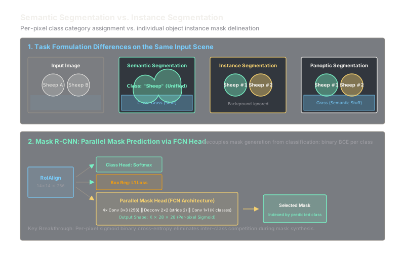
Semantic segmentation colors every pixel by category, while instance segmentation distinguishes individual objects of the same category.

Comparing semantic, instance, and panoptic segmentation outputs alongside Mask R-CNN binary mask generation.

Why Does This Exist?

Bounding box object detectors surround detected objects with axis-aligned rectangles. However, rectangular boxes are coarse approximations:

A pedestrian leaning against a lamppost shares substantial bounding box volume with the post, the sidewalk, and the background wall.
A robotic gripper attempting to pick a delicate metallic gear cannot rely on a loose box; it requires the gear's exact pixel boundaries to calculate grasp contact points.
Medical oncologists measuring tumor volumes or counting overlapping cell nuclei cannot tolerate box overlap.

Image segmentation solves this by elevating visual recognition to the pixel level. However, dense prediction splits into two distinct visual tasks with fundamentally different architectural requirements:

Semantic Segmentation: Classifies every single pixel in the image into a predefined semantic category (e.g., road, sky, car, person). If two cars overlap or touch, semantic segmentation merges them into a single continuous "car" blob without distinguishing individual vehicles.
Instance Segmentation: Simultaneously detects individual objects (things) and delineates a unique binary mask for each instance. It distinguishes between Car #1 and Car #2, but typically ignores amorphous background regions like sky or vegetation (stuff).

Panoptic segmentation unifies both: assigning a semantic class to every pixel while assigning unique instance IDs to all countable objects.

Think of It Like This

Coloring a map vs. issuing numbered passport photos

Imagine reviewing a high-altitude satellite photograph of a park filled with trees and visitors.

Semantic segmentation is a color-by-numbers cartographer. The cartographer takes a set of colored crayons: green for grass, brown for trees, blue for lakes, and orange for pedestrians. Every square millimeter of the map receives a crayon color. If ten people stand together in a tight circle playing music, the entire group is shaded with one unbroken patch of orange. You know where the "human" mass is located, but you cannot count how many people are in the circle.

Instance segmentation is an event photographer tagging visitors. The photographer ignores the continuous grass and sky entirely. Instead, they find Person #1, paste a clean silhouette cutout over their exact outline, and assign them ID badge #101. Then they trace Person #2 with badge #102, even if the two visitors are shaking hands. Every countable individual receives their own independent mask.

How It Actually Works

Semantic Segmentation Mechanics: Fully Convolutional Networks (FCNs)

Semantic segmentation treats the task as dense $K$ -class classification across an image $X \in \mathbb{R}^{3 \times H \times W}$ . Architectures such as FCN, DeepLab, and PSPNet eliminate fully connected layers in favor of an encoder-decoder structure:

Encoder: Consecutive convolutional and downsampling operations extract high-level semantic context while reducing spatial resolution by a factor of 8, 16, or 32.
Atrous / Dilated Convolutions: Expand filter receptive fields without losing spatial resolution by inserting spaces ( $r - 1$ zeros) between kernel elements:

y[i] = \sum_{k=0}^{K-1} x[i + r \cdot k] \cdot w[k]

Decoder: Bilinear upsampling, transpose convolutions, or Atrous Spatial Pyramid Pooling (ASPP) restore feature maps back to $H \times W \times K$ .
Per-pixel Softmax Loss: Computes multi-class cross-entropy independently for every pixel location $(i, j)$ :

\mathcal{L}_{\text{semantic}} = -\frac{1}{H \cdot W} \sum_{i=1}^{H} \sum_{j=1}^{W} \sum_{k=1}^{K} y_{i, j, k} \log \hat{p}_{i, j, k}

Instance Segmentation Mechanics: Mask R-CNN

Mask R-CNN (He et al., 2017) extended Faster R-CNN by adding a third parallel output branch: the mask branch.

For each candidate region of interest (RoI) generated by the RPN:

RoIAlign: Crops and resamples a fixed $14 \times 14$ feature patch from the backbone pyramid using bilinear interpolation. Unlike older RoI Pooling, RoIAlign avoids coordinate quantization, preserving sub-pixel spatial fidelity essential for mask outlines.
Classification & Box Head: Standard dense layers predict discrete class probabilities and box coordinate deltas.
Mask Branch (FCN): Applies four consecutive $3 \times 3$ convolutions (256 channels), followed by a $2 \times 2$ transposed convolution (stride 2) that upsamples spatial resolution to $28 \times 28$ . A final $1 \times 1$ convolution outputs a tensor of shape:

\mathbf{M} \in \mathbb{R}^{K \times 28 \times 28}

where $K$ is the number of target classes.

The Decoupling Principle: Per-Pixel Sigmoid Binary Loss

A foundational breakthrough of Mask R-CNN was decoupling mask generation from class competition.

If the mask branch used a spatial Softmax across classes, the model would force classes to compete at each pixel. Instead, Mask R-CNN applies a per-pixel Sigmoid independently to each of the $K$ channels. The mask loss is defined as average binary cross-entropy (BCE) evaluated only on the ground-truth class $k^*$ :

\mathcal{L}_{\text{mask}} = -\frac{1}{m^2} \sum_{i=1}^{m} \sum_{j=1}^{m} \left[ y_{i, j} \log \sigma(s_{i, j}^{k^*}) + (1 - y_{i, j}) \log(1 - \sigma(s_{i, j}^{k^*})) \right]

Other class masks $k \neq k^*$ contribute zero loss. Class prediction is handled entirely by the dedicated classification head, allowing the mask branch to focus purely on spatial object boundaries.

Worked Example

Let us compute the binary cross-entropy mask loss for a tiny $2 \times 2$ mask prediction on a ground-truth object of class $k^* = 1$ (Dog):

Ground-truth binary mask $Y$ :

Y = \begin{bmatrix} 1 & 1 \\ 0 & 1 \end{bmatrix}

Predicted logits for class 1 from the mask head:

S^{k^*} = \begin{bmatrix} 2.0 & 1.0 \\ -1.0 & 0.0 \end{bmatrix}

Calculate Sigmoid probabilities $\sigma(z) = \frac{1}{1 + e^{-z}}$ :

$\sigma(2.0) = \frac{1}{1 + e^{-2}} \approx 0.8808$
$\sigma(1.0) = \frac{1}{1 + e^{-1}} \approx 0.7311$
$\sigma(-1.0) = \frac{1}{1 + e^{1}} \approx 0.2689$
$\sigma(0.0) = 0.5000$

Calculate per-pixel binary cross-entropy $\ell = -[y \log(p) + (1 - y) \log(1 - p)]$ :

Pixel (0, 0) ( $y=1$ ): $-\log(0.8808) \approx 0.1269$
Pixel (0, 1) ( $y=1$ ): $-\log(0.7311) \approx 0.3132$
Pixel (1, 0) ( $y=0$ ): $-\log(1 - 0.2689) = -\log(0.7311) \approx 0.3132$
Pixel (1, 1) ( $y=1$ ): $-\log(0.5000) \approx 0.6931$

Mean mask loss across all 4 pixels:

\mathcal{L}_{\text{mask}} = \frac{0.1269 + 0.3132 + 0.3132 + 0.6931}{4} = \frac{1.4464}{4} = 0.3616

Code

1import torch2import torch.nn as nn3import torch.nn.functional as F4
5class MaskHead(nn.Module):6    """Mask R-CNN FCN Mask Branch producing K x 28 x 28 binary masks."""7    def __init__(self, in_channels: int = 256, num_classes: int = 80) -> None:8        super().__init__()9        # 4 consecutive Conv 3x3 layers10        self.convs = nn.Sequential(11            nn.Conv2d(in_channels, 256, kernel_size=3, padding=1),12            nn.ReLU(inplace=True),13            nn.Conv2d(256, 256, kernel_size=3, padding=1),14            nn.ReLU(inplace=True),15            nn.Conv2d(256, 256, kernel_size=3, padding=1),16            nn.ReLU(inplace=True),17            nn.Conv2d(256, 256, kernel_size=3, padding=1),18            nn.ReLU(inplace=True)19        )20        # Deconvolution 2x2 with stride 2 upsamples 14x14 to 28x2821        self.upsample = nn.ConvTranspose2d(256, 256, kernel_size=2, stride=2)22        self.relu = nn.ReLU(inplace=True)23        # 1x1 conv to K mask channels24        self.classifier = nn.Conv2d(256, num_classes, kernel_size=1)25
26    def forward(self, x: torch.Tensor) -> torch.Tensor:27        x = self.convs(x)28        x = self.relu(self.upsample(x))29        return self.classifier(x)30
31# Input from RoIAlign: 4 candidate RoIs, 256 channels, 14x14 spatial size32roi_features = torch.randn(4, 256, 14, 14)33mask_head = MaskHead(in_channels=256, num_classes=80)34
35# Raw output logits: (Batch=4, Classes=80, Height=28, Width=28)36mask_logits = mask_head(roi_features)37print(mask_logits.shape)38# -> torch.Size([4, 80, 28, 28])

Watch Out For

Misalignment artifacts from naive RoI pooling and border clipping

In instance segmentation, sub-pixel alignment is critical. Standard RoI Pooling (used in original Fast R-CNN) rounds floating-point region proposals (e.g., $x=20.7 \to 20$ ) and rounds bin boundaries during pooling. While a 1-pixel shift has minor impact on a box classification score, it severely degrades mask IoU, cutting off object borders and blurring fine edges like human limbs.

Always verify that your architecture uses RoIAlign with bilinear interpolation rather than quantized RoI Pooling. Furthermore, when mapping the predicted $28 \times 28$ normalized mask back into original image space, resize the mask directly to the unrounded bounding box coordinates before binarizing at threshold $p \ge 0.5$ .

The Quick Version

Semantic segmentation labels every pixel by categorical class, merging overlapping instances of the same category into one continuous mask.
Instance segmentation identifies and segments individual object instances, distinguishing between adjacent or overlapping instances.
Panoptic segmentation combines semantic "stuff" (amorphous backgrounds) with instance "things" (countable objects).
Mask R-CNN adds a small FCN mask branch in parallel with standard Faster R-CNN box classification and regression heads.
Applying per-pixel Sigmoid binary cross-entropy decouples mask boundary generation from multi-class competition.