Video Prediction

The best test of understanding motion is predicting the next frames. Video prediction rolls the present forward: physics, intent, and camera motion compressed into future pixels.

One present splits into two futures, so the mean predictor paints a ghost at 7 while sampling stays sharp

Why Does This Exist?

Recognition names the present; action needs the future. A car must know where the pedestrian will be, not where they are; a robot must foresee the toppling tower before pushing. Simulation covers scripted cases, but the open world keeps inventing unscripted ones — prediction from raw video is the general fallback.

Video prediction is also the strictest unsupervised exam: any model can memorize textures, but only one that understands motion, physics, and intent predicts frames it never saw. That exam pressure produced the stochastic, patch-wise, and latent-rollout designs below. The loop it feeds is embodied vision; the dynamics conscience is physical reasoning.

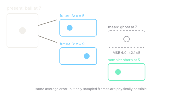
The one idea you need first. The future is multimodal: one present branches into many valid futures (the ball bounces left or right). A deterministic predictor trained with mean-squared error outputs the average of the branches — a blurry ghost sitting between real outcomes. Sharp prediction requires sampling one branch (stochastic latents) rather than averaging all of them.

Think of It Like This

Catching a ball with your eyes half closed

Fielders do not watch the ball land and then run; they predict the landing spot from the first half-second of flight and arrive with the mitt ready. The prediction fuses physics (gravity bends the arc), intent (the batter's swing), and camera motion (your own sprint) into one future position, updated every glance.

Video prediction is that catch computed in pixels. Deterministic models predict the average landing spot of every possible throw — a ghost point between fields. Stochastic models pick one throw and run there. Only the second fielder ever catches anything.

How It Actually Works

Three families split the problem by horizon and sharpness needs. Deterministic regressors (3D CNNs, recurrent predictors with MSE loss) give one future and blur under uncertainty — fine for tenths of a second. Stochastic models (VRNNs, diffusion forecasters) sample latent variables per step, keeping each sampled future sharp across seconds. Token autoregressors quantize patches or frames and predict tokens like language models, trading spatial fidelity for long horizons. Evaluation mixes pixel scores (PSNR, SSIM) with perceptual and task scores, because pixel metrics forgive semantic nonsense.

Error compounds with horizon in all families: each predicted frame feeds the next, so drift grows step by step.

Worked example

A ball sits at $x = 7$ and will be at $x = 5$ or $x = 9$ next frame, each with probability $0.5$ . The MSE-optimal single prediction is the mean, $7$ :

$\text{MSE} = 0.5(7-5)^2 + 0.5(7-9)^2 = 0.5 \times 4 + 0.5 \times 4 = 4.0$

On a $0$ – $255$ scale that is $\text{PSNR} = 10\log_{10}(255^2/4) = 10\log_{10}(16{,}256) \approx 42.1$ dB — a respectable number for a ghost ball sitting where no future goes. A stochastic model sampling one branch scores $0$ error half the time and $16$ the other half: same average, but every sample is a physically possible frame.

Code

The point of this snippet is the ghost arithmetic: the mean minimizes MSE while painting an impossible frame.

1import math2
3
4def psnr(mse: float, max_val: float = 255.0) -> float:5    return 10.0 * math.log10(max_val**2 / mse)  # dB, higher is better6
7
8mse_mean = 0.5 * (7 - 5) ** 2 + 0.5 * (7 - 9) ** 29print(mse_mean)  # -> 4.010print(round(psnr(mse_mean), 1))  # -> 42.1

Watch Out For

Blur mistaken for the model ceiling

MSE-trained predictors blur, and teams read the blur as "prediction is just hard" rather than as a loss-function artifact. The same architecture with a stochastic head or adversarial loss stays sharp on identical data — the ceiling was the objective, not the problem.

Diagnose before scaling: if samples average to the prediction (ghost check), the loss is averaging futures. Switch the objective before blaming capacity.

Horizons that outrun the error budget

Single-step error $\epsilon$ compounds roughly linearly at first, then superlinearly as predictions feed predictions: ten steps at $\epsilon$ each rarely cost $10\epsilon$ . Demos showing thirty sharp frames usually cherry-pick the seed or the clip.

Report error-versus-horizon curves, not best frames. Plan with the horizon the curve supports (often under a second for pixels, longer for latent rollouts), and re-observe instead of open-looping past it.

The Quick Version

Video prediction rolls present frames into future ones, examing motion, physics, and intent understanding.
Multimodal futures punish deterministic predictors: the mean of branches is a ghost no future visits.
The worked fixture gives MSE $4.0$ and PSNR $42.1$ dB for a ghost prediction at $x = 7$ .
Stochastic latents and token autoregression keep samples sharp across longer horizons.
Blur usually indicts the MSE objective, not model capacity — run the ghost check first.
Error compounds with horizon, so report curves and re-observe past the supported range.