ARIMA
The classic time series algorithm that forecasts the future by combining the momentum of past values (AutoRegressive) with the momentum of past errors (Moving Average), after stabilizing the data (Integrated).
Why Does This Exist?
In the early days of statistics, there were two competing theories for how to forecast a time series.
The first camp believed in AutoRegression (AR): "To predict tomorrow's stock price, just look at the price from the last 3 days and draw a line." The second camp believed in Moving Averages (MA): "To predict tomorrow, look at how wrong our predictions were over the last 3 days (the errors), and correct for them."
In 1970, statisticians Box and Jenkins proved that combining both approaches created a vastly superior model. They added an "Integrated" (I) step to enforce Stationarity, and the ARIMA model was born. It remained the undisputed king of forecasting for 40 years until gradient boosting and deep learning arrived.
Think of It Like This
Think of It Like This
Imagine you are steering a large ship into a harbor.
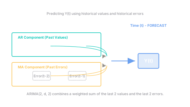
AR (AutoRegressive) is your momentum. If you have been moving left for the last three seconds, your momentum dictates you will probably continue moving left in the next second.
MA (Moving Average) is your course correction. You notice that your last three steering adjustments over-corrected, pushing you slightly off course (the errors). You mathematically subtract those past errors from your current steering to ensure a smooth docking.
ARIMA combines your current momentum with your past mistakes to calculate the perfect trajectory.
How It Actually Works
ARIMA is defined by three parameters: .
1. The I-term (): Integration (Differencing)
ARIMA requires strict stationarity. If your data is trending upwards, ARIMA will fail. The parameter tells the model how many times to apply differencing (subtracting from ) to force the data to become flat. Usually, .
2. The AR-term (): AutoRegressive
This tells the model how many past days (lags) to look at. If , the formula to predict tomorrow includes a weighted sum of yesterday and the day before. We determine the value of by looking at the PACF plot.
3. The MA-term (): Moving Average
This is the hardest part to understand. It does not mean the classical moving average indicator you see on stock charts. It refers to the past forecast errors (). If , the model calculates how wrong it was yesterday, and factors that error into today's prediction to auto-correct itself. We determine by looking at the ACF plot.
The full ARIMA model simply adds these equations together.
SARIMA (Seasonal ARIMA)
Standard ARIMA cannot handle seasonality (e.g., spikes that happen every 12 months). To fix this, statisticians created SARIMA, which adds three more parameters . It essentially runs a second, parallel ARIMA model that jumps back steps at a time (e.g., looking at exactly this month last year).
Code
In Python, statsmodels is the standard library for ARIMA. However, determining the exact parameters manually via ACF/PACF plots is tedious. Modern practitioners use the pmdarima library, which provides an auto_arima function that tests hundreds of combinations and automatically selects the best one (similar to R's famous auto.arima).
import pandas as pdimport pmdarima as pm
# A dataset of monthly airline passengers (highly seasonal)# Since it is monthly, seasonal period m=12data = pd.read_csv('airline_passengers.csv', index_col='Month')
# Run Auto-ARIMA to automatically find the best (p,d,q) and (P,D,Q)# It uses the AIC metric to score the modelsmodel = pm.auto_arima( data['Passengers'], seasonal=True, m=12, trace=True, # Prints the models it tries error_action='ignore', suppress_warnings=True)
print(model.summary())
# Forecast the next 12 monthsforecast, conf_int = model.predict(n_periods=12, return_conf_int=True)print("\nForecast for next year:\n", forecast)Watch Out For
It cannot use external features easily.
ARIMA only looks at its own history. If you want to predict umbrella sales, the most important feature is "Is it raining tomorrow?". Standard ARIMA cannot ingest a weather forecast. You must upgrade to ARIMAX (ARIMA with eXogenous variables), but even then, it struggles with non-linear relationships compared to models like XGBoost.
The Quick Version
- ARIMA is a classical statistical model for forecasting time series.
- AR (p): Uses past values to predict the future (momentum).
- I (d): Differences the data to make it stationary (flat).
- MA (q): Uses past forecast errors to correct the future trajectory.
- Standard ARIMA cannot handle repeating cycles; you must use SARIMA to model seasonality.
- While it has been largely superseded by gradient boosting for complex business datasets, it remains an extremely fast and powerful baseline.