Core ML

Continual Learning

Train on a new task and the old one collapses, because nothing in the new gradient knows the old loss exists. Every fix is a form of don't move too far.

Training on a second task drives accuracy on the first one down to chance, and mixing a small buffer of old examples into every batch holds most of it

Why Does This Exist?

A helpdesk router sorts tickets into forty queues. Live for two years, and good. Then the company launches a product line, six new queues appear, and you have four thousand tickets for them.

Retraining from scratch means rebuilding on two years of data every quarter, so the obvious move is to keep training the model you have on the new tickets. It works — the six new queues route beautifully.

And accuracy on the original forty falls off a cliff. Not a few points of drift — roughly where you'd land sending every ticket to the biggest queue. This is catastrophic forgetting, and the name is accurate rather than dramatic.

The reason is mechanical, and it makes every mitigation predictable. The gradient you compute on the new tickets is the gradient of the new loss. That's it. Nothing refers to the old queues, no penalty exists for moving a weight the old task needed. Worse than neutral, in fact: the weights that mattered most to the old queues carry the most useful signal for the new ones, so those move first.

Think of It Like This

One guitar, two tunings

You know a song in standard tuning. A friend wants one in open D, so you turn three pegs and play it. Sounds great.

Now play the first song. It's gone. Not rusty in your fingers — physically unavailable, the strings are somewhere else. And nothing about turning those pegs consulted the first song. No force resisted you.

Three ways out, each one billing you. Keep checking the old song as you retune and accept a compromise tuning that plays neither perfectly. Fit stiffer pegs, protecting the old tuning and making the new one harder to reach by exactly the same stiffness. Or buy a second guitar, which forgets nothing and costs a second guitar.

How It Actually Works

Why it collapses instead of degrading

A network's knowledge of a task isn't in a labelled compartment. It's spread across weights every other task also uses, so there's no overwriting ten percent of it. Move a shared weight far enough and the whole decision boundary that depended on it moves.

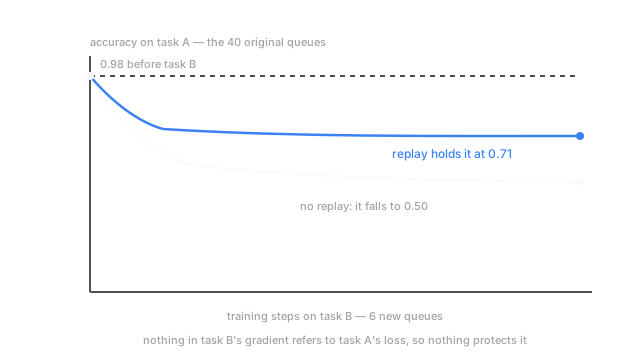
That's why the diagram's curve falls the way it does. The new task's optimum sits where the old task's accuracy is near chance, gradient descent walks straight to it, and nothing on the route treats the old loss as a cost. Continual learning adds that cost back without freezing the model so hard it can't learn.

Three answers to the same question

Replay keeps a buffer of old examples and mixes them into every batch. Now the gradient genuinely contains a term for the old task, because some of the batch is the old task. Most direct fix, works best. The blocker is rarely technical: retention policy, deletion requests and data agreements decide whether you can keep the tickets.

Regularisation keeps no data. It penalises movement in weights the earlier task needed:

\mathcal{L}(\theta) = \mathcal{L}_{B}(\theta) + \frac{\lambda}{2}\sum_{i} F_{i}\left(\theta_{i} - \theta_{A,i}\right)^{2}

$\mathcal{L}_{B}$ is the loss on the new task, $\theta_{i}$ is weight $i$ right now, $\theta_{A,i}$ what it was when the old task finished, $F_{i}$ estimates how much that weight mattered to the old task, and $\lambda$ is how hard you hold on. It's weight decay, except it pulls toward the old weights instead of zero, and each weight gets its own strength. $F_{i}$ comes from the curvature of the old loss: steep curvature means moving that weight hurts, so hold it still.

Architectural approaches give each task its own parameters: an adapter per task, a mask routing each task through its own subnetwork, or a new model. Forgetting drops to zero by construction. The cost is a parameter count growing with every task, and knowing which task you're serving.

Which one to reach for

Replay with a modest buffer beats most sophisticated alternatives. That's the field's least glamorous and most reproducible finding, and your baseline before anything with a Fisher matrix in it.

Everything here hits the same wall, the stability-plasticity tension. Every mechanism that protects old knowledge resists weight movement, and new learning is weight movement. No setting gets you both — you're choosing where on that curve to sit, and that choice should be explicit rather than a default.

Show Me the Code

Two linear tasks reading disjoint halves of the input. Train A, then B, and watch A go.

1import numpy as np2
3def train(x: np.ndarray, y: np.ndarray, w: np.ndarray, steps: int = 600) -> np.ndarray:4    for _ in range(steps):      # nothing in this gradient knows task A's loss exists5        w = w - 0.5 * x.T @ (x @ w - y) / len(y)6    return w7
8def acc(w: np.ndarray, x: np.ndarray, y: np.ndarray) -> float:9    return float((np.sign(x @ w) == y).mean())10
11rng = np.random.default_rng(0)12xa, xb = rng.normal(size=(240, 20)), rng.normal(size=(240, 20))13ya = np.sign(xa @ np.concatenate([rng.normal(size=10), np.zeros(10)]))  # A reads cols 0-914yb = np.sign(xb @ np.concatenate([np.zeros(10), rng.normal(size=10)]))  # B reads cols 10-1915w_a = train(xa, ya, np.zeros(20))16bx = np.vstack([xb, np.tile(xa[:24], (10, 1))])   # 24 kept rows, replayed 1:1 against B17by = np.concatenate([yb, np.tile(ya[:24], 10)])18w_r = train(bx, by, w_a)19print(f"task A: {acc(w_a, xa, ya):.2f} -> {acc(train(xb, yb, w_a), xa, ya):.2f} plain, {acc(w_r, xa, ya):.2f} replayed")20print(f"task B lands at {acc(w_r, xb, yb):.2f} with replay, {acc(train(xb, yb, w_a), xb, yb):.2f} without")21# -> task A: 0.98 -> 0.50 plain, 0.71 replayed22# -> task B lands at 0.73 with replay, 0.96 without

Task A falls from 0.98 to 0.50, a coin flip on two classes — the columns it depended on were noise for B, so least squares drove them to zero. Twenty-four kept rows pull it back to 0.71, and B lands at 0.73 instead of 0.96. There's the tension.

Watch Out For

Measuring only the task you just trained on

The quarterly retrain finishes, new-queue accuracy looks strong, the dashboard is green, and nobody notices for six weeks. Not carelessness — the metric you reach for after an update is the one that structurally cannot see the problem.

Evaluate on every earlier task after every stage. Keep a held-out set per task and report the whole matrix: rows are training stages, columns are tasks, and the diagonal is all your current metric shows you. The one number worth a dashboard slot is average accuracy across all tasks so far — it drops the moment an old task breaks.

Treating a small replay buffer as free

You cap the buffer at 5,000 tickets and fill it with the most recent, because recency seems sensible. Six months later the rare queues — legal escalations, hardware recalls, where a misroute is expensive — have aged out entirely, and the model has forgotten the classes you could least afford to lose.

A buffer isn't storage. It's a decision about what survives, made once and applied silently every quarter after. Sample it class-balanced so every queue keeps a floor of examples regardless of volume, or score by loss contribution and keep the informative ones. Then count examples per class against what you want the model to still do — stratified sampling is the right default.

The Quick Version

Train on task B after task A and A's accuracy collapses toward chance. Mechanical: B's gradient contains no term for A's loss.
It collapses rather than degrades because knowledge lives in shared weights, so you can't overwrite a fraction.
Replay mixes buffered old examples into new batches. Most effective, and the blocker is usually data retention, not engineering.
Regularisation penalises movement in weights the old task needed, using loss curvature as the importance estimate.
Architectural methods give each task its own parameters. Zero forgetting, unbounded growth.
Stability and plasticity trade off directly, so pick your point on that curve deliberately.