Core ML

Weight Decay

Adding a squared-size penalty to the loss is the same as multiplying every weight by a shade under one each step. That equality breaks under Adam, so AdamW.

Two fits through the same six measurements: large weights buy an exact pass through every point at the cost of a slope about six times steeper, while smaller weights give up the exact fit for a function that barely moves when the input does

Why Does This Exist?

You can draw endlessly many curves through the same handful of dots. Most are terrible.

A near-infrared scanner reads 200 wavelengths off a crate of apples, and a small network turns those numbers into a sugar reading in Brix. You have 60 labelled crates, because measuring true sugar means destroying the fruit. It fits — gradient descent drives training error to almost nothing. The question is how.

Here's the wall. One weight comes back at +412, the wavelength next door at −398, nearly cancelling. Two adjacent channels of a spectrum are almost the same measurement, so the network used the difference between two near-identical numbers as a free parameter. That works until the scanner drifts: three parts in a thousand on one channel moves the prediction by more than a full Brix, the difference between shipping a crate and holding it.

Think of It Like This

Forcing a steel spline through the pins

Draughtsmen drew smooth curves with a spline: a thin steel strip bent to pass through a row of pins on the board.

A very thin strip goes through every pin, whipping off in wild arcs between them, two inches from anywhere sensible halfway along. A thicker strip fights you: it passes near the pins, misses a couple by a millimetre, stays smooth. The bending energy it costs to force a curve is what stops the curve being ridiculous.

Weight decay is the strip's thickness. Notice what thickness doesn't stop — sliding the whole strip an inch left costs no bending energy. Bending is penalised, sliding is free, and that's why some parameters belong in the penalty and some don't.

How It Actually Works

The penalty and the multiplication are the same move

L_{\text{total}}(w) = L(w) + \frac{\lambda}{2}\lVert w \rVert^{2} \qquad\Longrightarrow\qquad w \leftarrow (1 - \eta\lambda)\,w - \eta\,\nabla L(w)

$w$ is every weight stacked into one vector, $L$ the ordinary loss, $\lVert w \rVert^{2}$ the sum of every weight squared — the squared L2 norm. $\lambda$ sets the decay strength, $\eta$ the learning rate.

Left to right is one line of algebra. The penalty's derivative for any single weight is $\lambda w$ , proportional to that weight's own size, so a step subtracts $\eta\lambda w$ before anything the data asked for. Collect the $w$ terms: multiply every weight by $1 - \eta\lambda$ , then take the ordinary step. At $\eta = 0.1$ and $\lambda = 0.05$ that's 0.995 — half a percent off every weight, every step. That multiplication is the decay in the name.

A weight settles where the pull toward zero balances the pull from the data, so weights the data doesn't care about drift to nearly nothing. Ridge regression has that with closed-form algebra.

What smoothness buys inside a network

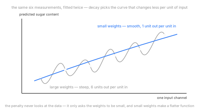
A network's output responds to an input change roughly in proportion to the product of the weight magnitudes on the path between them. Halve every weight in a two-layer network and the output moves about a quarter as much per unit of input. Small weights mean a flatter function — not less expressive, less sensitive.

Which is what generalisation wants: next season's apples aren't this season's, and the scanner will drift. A slope of 6 Brix per unit of reflectance turns a small input difference into a big one; a slope of 1 doesn't.

Why Adam needed AdamW, and what to exclude

Adam divides each parameter's update by a running estimate of its recent gradient sizes — the second moment — so big-gradient parameters take small steps. Put the penalty in the loss and it becomes part of the gradient, so it goes through that division.

The decay a weight receives is therefore $\eta\lambda w$ divided by the root of its own second moment, so the strength you set is not the strength you get. AdamW applies the shrinkage straight to the parameters, outside the adaptive step.

What to leave out: biases, because a bias only shifts the function up or down, so shrinking one makes nothing smoother and drags predictions toward zero. Also normalisation's learned scale and shift — pulling a learned scale toward zero fights the layer's job.

One consequence is genuinely surprising. When a layer's output is normalised, multiplying its incoming weights by any positive constant changes nothing — normalisation divides it back out. Decay there removes no capacity; it shrinks magnitude, and a scale-invariant layer's gradient falls as weights grow, so smaller magnitude means a relatively larger step. Decay moves the effective learning rate.

Show Me the Code

Four weights of identical size, four gradient scales, and the pull toward zero each one actually receives.

1import numpy as np2
3
4def shrinkage(w: np.ndarray, lam: float, lr: float, v: np.ndarray) -> np.ndarray:5    return lr * lam * w / (np.sqrt(v) + 1e-8)  # v is 1 for SGD, the second moment for Adam6
7
8w: np.ndarray = np.full(4, 0.9)  # four weights of identical size9g: np.ndarray = np.array([0.01, 0.1, 1.0, 10.0])  # but wildly different gradient scales10
11print("penalty in the loss, SGD ", np.round(shrinkage(w, 0.05, 0.1, np.ones(4)), 5))12print("penalty in the loss, Adam", np.round(shrinkage(w, 0.05, 0.1, g ** 2), 5))13print("decoupled, AdamW         ", np.round(0.1 * 0.05 * w, 5))14# -> penalty in the loss, SGD  [0.0045 0.0045 0.0045 0.0045]15# -> penalty in the loss, Adam [0.45    0.045   0.0045  0.00045]16# -> decoupled, AdamW          [0.0045 0.0045 0.0045 0.0045]

Under plain gradient descent every weight gets the same 0.0045 pull. Send the identical penalty through Adam's division and the sleepiest weight gets 0.45 — a hundred times the intended pull — the busiest 0.00045. One $\lambda$ , a thousand-fold spread.

Watch Out For

One parameter group, decay on everything

Nothing breaks, which is what makes this expensive. Accuracy sits a point or two below what the same recipe reaches elsewhere, with no error to chase. Usually one line: AdamW(model.parameters(), weight_decay=0.01) hands the optimiser a single group, so every bias and normalisation scale gets shrunk with the weight matrices.

The fix is two groups. Anything whose name ends in bias, plus every normalisation weight, goes into a group with weight_decay=0.0. Verify rather than assume — defaults differ between libraries, and a training wrapper can quietly collapse your groups into one.

Carrying a decay value between SGD and AdamW

You lift weight_decay=0.0001 out of a well-tuned SGD recipe, drop it into AdamW, and the model overfits as though there were no penalty. Go the other way with 0.01 and it never gets off the floor.

The number means different things in the two places. Under SGD the penalty enters through the gradient and then the momentum buffer, so at momentum 0.9 the accumulated shrinkage is roughly ten times $\eta\lambda$ ; under AdamW it lands on the parameter at exactly $\eta\lambda$ . SGD also runs a learning rate near 0.1 against AdamW's 0.001, so the same $\lambda$ lands orders of magnitude apart. Conventional values reflect it: 0.0001 to 0.0005 for SGD on vision, 0.01 to 0.1 for AdamW on transformers.

The Quick Version

The penalty's gradient is proportional to each weight's size, so under plain gradient descent it's the same as multiplying every weight by $1 - \eta\lambda$ each step.
Smaller weights mean the output changes less per unit of input, and that smoothness is what generalisation wants.
Adaptive optimisers divide the penalty by the second moment, so the strength you set isn't the strength you get. AdamW applies it to the parameters instead.
Exclude biases and normalisation scale-and-shift parameters. Two parameter groups, not one.
Under a normalisation layer, decay on the incoming weights changes no function — it moves the effective learning rate.
Decay values don't transfer between SGD and AdamW recipes.