Dropout DropConnect Stochastic Depth

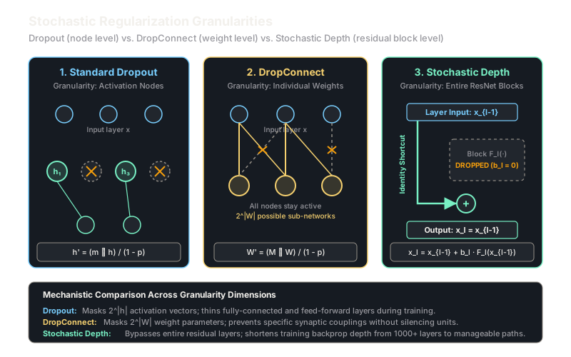
Stochastic regularization zeroes out activations, weights, or entire residual blocks during training to destroy fragile co-adaptations. It forces deep networks to operate as exponential ensembles of thinned subnetworks.

Stochastic regularization suppresses over-reliance by randomly zeroing activations, individual weight connections, or complete residual blocks during training.

Why Does This Exist?

Deep neural networks with millions or billions of parameters possess sufficient capacity to memorize training datasets completely, fitting random noise rather than generalizable data patterns. In standard dense networks, features develop mutual co-adaptations: one hidden unit learns to correct the idiosyncratic mistake of another, creating fragile dependencies that collapse when presented with out-of-distribution test samples.

Conventional deterministic regularization techniques like $L_2$ weight decay penalize large weight magnitudes, but they do not disrupt structural co-adaptation. If five hidden units collaborate to memorize an atypical edge case, weight decay merely shrinks their coefficients slightly without forcing them to discover independently useful representations. Furthermore, in ultra-deep networks spanning hundreds of layers, gradient attenuation stalls early layers during optimization.

Stochastic regularization methods inject random Bernoulli noise into the network during training, sampling a different subnetwork for every minibatch. By varying the structural granularity of this randomness—from individual activation nodes (dropout) to synaptic connections (DropConnect) to entire macro-residual blocks (Stochastic Depth)—practitioners eliminate fragile feature dependencies and dramatically stabilize deep architectures.

Think of It Like This

A cross-training sports team with unannounced absences

Imagine an elite rowing team preparing for a championship. If the exact same eight rowers practice in identical seat assignments every afternoon, subtle compensations develop: the rower in seat three might slack off slightly because seat four over-pulls to compensate. The crew appears synchronized, but if seat four suffers an injury, the boat veers off course.

To prevent this fragile dependency, the head coach introduces unannounced practice drills across three levels:

First, random rower absences (Dropout): on any practice day, two random rowers are benched, forcing the remaining crew to row evenly without relying on specific teammates.

Second, random paddle swaps (DropConnect): all rowers remain in the boat, but specific mechanical couplings between individual rowers and their oars are swapped or silenced at random, forcing rowers to handle diverse stroke resistances.

Third, shortened course segments (Stochastic Depth): during an endurance marathon across twenty consecutive river locks, the coach randomly lifts entire rowing sections out of the water, forcing the team to sprint through varying subsets of the total course without fatiguing the core boat hull.

How It Actually Works

Granularities of Stochastic Thinning

Stochastic regularization techniques differ fundamentally in the mathematical tensor level at which the Bernoulli mask is applied.

1. Standard Inverted Dropout (Node Level)

Dropout zeroes out hidden activation vectors $h \in \mathbb{R}^d$ with drop probability $p \in [0, 1)$ (retention probability $q = 1 - p$ ). In modern deep learning frameworks, inverted dropout applies scaling during the forward pass of training so that test-time evaluation requires no architectural modification:

m \sim \text{Bernoulli}(1 - p), \quad h_{\text{train}} = \frac{m \odot h}{1 - p}

Because $\mathbb{E}[m_i] = 1 - p$ , the scaling factor $\frac{1}{1 - p}$ ensures that the expectation is preserved between training and inference:

\mathbb{E}[h_{\text{train}}] = \frac{\mathbb{E}[m] \odot h}{1 - p} = \frac{(1 - p) h}{1 - p} = h = h_{\text{test}}

Dropout implicitly averages an ensemble of $2^d$ distinct thinned sub-architectures sharing parameter weights.

2. DropConnect (Weight/Connection Level)

Introduced by Wan et al. (2013), DropConnect generalizes Dropout by applying the stochastic mask directly to the parameter weight matrix $W \in \mathbb{R}^{d_{\text{out}} \times d_{\text{in}}}$ rather than the output activations:

M_{ij} \sim \text{Bernoulli}(1 - p), \quad W_{\text{train}} = \frac{M \odot W}{1 - p}

z = W_{\text{train}} x + b

While Dropout sets entire rows or columns of active incoming signals to zero, DropConnect allows any hidden unit to remain active as long as at least one of its incoming synaptic weights survives. This expands the ensemble space from $2^{|h|}$ possible sub-states to $2^{|W|}$ possible connection topologies.

3. Stochastic Depth (Residual Block Level)

Introduced by Huang et al. (2016) for ultra-deep residual networks (ResNets), Stochastic Depth operates macroscopically. In a residual network, layer $l$ computes:

x_l = x_{l-1} + f_l(x_{l-1})

Stochastic Depth introduces a scalar Bernoulli random variable $b_l \in \{0, 1\}$ with survival probability $p_l$ :

x_l = x_{l-1} + b_l \cdot f_l(x_{l-1})

When $b_l = 0$ , the non-linear residual branch $f_l$ is bypassed entirely, reducing the block to an exact identity mapping $x_l = x_{l-1}$ . The survival probability typically follows a linear decay schedule across layer depth $l \in [1, L]$ :

p_l = 1 - \frac{l}{L}(1 - p_L)

Early layers that extract fundamental low-level features are retained with high probability ( $p_0 = 1.0$ ), while deeper layers drop frequently. During training, the expected path length drops significantly, accelerating forward and backward passes. At test time, all blocks are active and calibrated by their survival probability: $x_l = x_{l-1} + p_l f_l(x_{l-1})$ .

Worked Example

Let an input vector $x = [2.0, -1.0]^\top$ pass through a linear layer with weight matrix $W$ and bias $b = [0.0, 0.0]^\top$ :

W = \begin{bmatrix} 0.5 & -0.4 \\ 1.0 & 0.8 \end{bmatrix}

Let retention probability $q = 1 - p = 0.5$ , yielding an inverted scaling multiplier $\frac{1}{q} = \frac{1}{0.5} = 2.0$ .

Forward Step 1: Pre-activation Without Regularization

z_1 = (0.5 \times 2.0) + (-0.4 \times -1.0) = 1.0 + 0.4 = 1.4

z_2 = (1.0 \times 2.0) + (0.8 \times -1.0) = 2.0 - 0.8 = 1.2

With $\text{ReLU}(z)$ , hidden state $h = [1.4, 1.2]^\top$ .

Forward Step 2: Standard Inverted Dropout

Sample mask $m = [1, 0]^\top$ (node 1 retained, node 2 dropped):

h_{\text{drop}} = \frac{1}{0.5} (m \odot h) = 2.0 \times [1.4 \times 1, 1.2 \times 0]^\top = [2.8, 0.0]^\top

The expected activation $\mathbb{E}[h_{\text{drop}}] = 0.5 \times [2.8, 0.0]^\top + 0.5 \times [0.0, 2.4]^\top = [1.4, 1.2]^\top = h$ .

Forward Step 3: DropConnect

Sample weight mask $M$ :

M = \begin{bmatrix} 1 & 0 \\ 1 & 1 \end{bmatrix}

Scale and mask weights:

W_{\text{train}} = 2.0 \times (M \odot W) = \begin{bmatrix} 2.0 \times 0.5 & 2.0 \times 0.0 \\ 2.0 \times 1.0 & 2.0 \times 0.8 \end{bmatrix} = \begin{bmatrix} 1.0 & 0.0 \\ 2.0 & 1.6 \end{bmatrix}

Compute output:

z_{\text{dc}} = W_{\text{train}} x = \begin{bmatrix} 1.0(2.0) + 0.0(-1.0) \\ 2.0(2.0) + 1.6(-1.0) \end{bmatrix} = \begin{bmatrix} 2.0 \\ 4.0 - 1.6 \end{bmatrix} = \begin{bmatrix} 2.0 \\ 2.4 \end{bmatrix}

Notice that both output neurons remain non-zero even though individual synaptic connections were dropped.

Code

1import numpy as np2
3def inverted_dropout(4    h: np.ndarray,5    p_drop: float,6    training: bool = True7) -> np.ndarray:8    """Apply inverted dropout to activation tensor h."""9    if not training or p_drop == 0.0:10        return h11    q = 1.0 - p_drop12    mask = (np.random.rand(*h.shape) < q).astype(np.float64)13    return (h * mask) / q14
15def dropconnect_forward(16    x: np.ndarray,17    W: np.ndarray,18    p_drop: float,19    training: bool = True20) -> np.ndarray:21    """Apply DropConnect to weight matrix W during forward pass."""22    if not training or p_drop == 0.0:23        return np.dot(W, x)24    q = 1.0 - p_drop25    mask = (np.random.rand(*W.shape) < q).astype(np.float64)26    w_effective = (W * mask) / q27    return np.dot(w_effective, x)28
29def stochastic_depth_block(30    x: np.ndarray,31    residual_fn,32    p_survival: float,33    training: bool = True34) -> np.ndarray:35    """Pass input through residual block with stochastic depth."""36    if not training:37        return x + p_survival * residual_fn(x)38    survives = np.random.rand() < p_survival39    if not survives:40        return x  # Identity bypass41    return x + (1.0 / p_survival) * residual_fn(x)42
43# Reproducible test case44np.random.seed(42)45h_test = np.array([1.4, 1.2], dtype=np.float64)46w_test = np.array([[0.5, -0.4], [1.0, 0.8]], dtype=np.float64)47x_in = np.array([2.0, -1.0], dtype=np.float64)48
49# Deterministic evaluation (inference mode)50h_eval = inverted_dropout(h_test, p_drop=0.5, training=False)51y_eval = dropconnect_forward(x_in, w_test, p_drop=0.5, training=False)52
53print(f"Eval Dropout: {h_eval.tolist()}")54# -> Eval Dropout: [1.4, 1.2]55
56print(f"Eval DropConnect: {y_eval.tolist()}")57# -> Eval DropConnect: [1.4, 1.2]

Watch Out For

Forgetting to toggle eval mode causes test-time prediction variance and metric degradation

A widespread practitioner error is failing to disable stochastic masks during evaluation (e.g., forgetting model.eval() in PyTorch).

If dropout or stochastic depth remains active during testing, the network outputs stochastic predictions for the identical input across different inference calls. Because single inference runs only sample a single thinned subnetwork without inverted ensemble aggregation, test-set classification error surges and benchmark metrics degrade sharply. Always ensure evaluation harnesses explicitly switch models into deterministic evaluation mode.

The Quick Version

Standard Dropout zeros out hidden activation units, DropConnect zeros out individual connection weights, and Stochastic Depth bypasses entire residual blocks.
Inverted dropout divides surviving activations by the retention probability $(1 - p)$ during training, eliminating any test-time computational overhead.
Stochastic Depth enables the stable training of ultra-deep networks spanning over 1,000 layers by shortening the effective backpropagation path.