Embeddings and Word Representations

Dense numerical vectors that map discrete vocabulary tokens into a continuous geometric space. Words with similar contextual usage cluster together and preserve linear relational analogies.

Embeddings project discrete orthogonal one-hot tokens into a dense continuous space where semantic relations emerge as spatial distances and directional offsets.

Why Does This Exist?

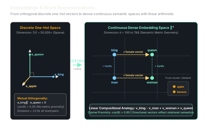
In classical natural language processing, words were treated as atomic, indivisible symbols. Under a one-hot encoding across a vocabulary of size $|V| = 50,000$ , every distinct word is represented as a 50,000-dimensional sparse unit vector containing a single 1 and 49,999 zeros.

This discrete representation suffers from two catastrophic mathematical limitations. First, memory scale: maintaining and computing transformations across high-dimensional sparse vectors creates massive matrix multiplications. Second, metric blindness: because every one-hot vector is perpendicular to every other vector, the inner product $e_i^\top e_j = 0$ for all $i \ne j$ , and the Euclidean distance $\|e_i - e_j\|_2 = \sqrt{2}$ . The vector for "doctor" is just as distant from "physician" as it is from "sandpaper". A statistical model trained on sentences about "physicians" cannot generalize to "doctors" without explicit co-occurrence data.

Dense word embeddings solve this by mapping discrete tokens into a continuous low-dimensional vector space $\mathbb{R}^d$ ( $d \ll |V|$ , typically 100 to 768). In this continuous space, geometric proximity mirrors semantic relatedness, and linear spatial translations correspond to semantic transformations, providing foundational inputs for multi-layer perceptrons and transformers.

Think of It Like This

A spatial town map versus an unorganized filing cabinet

Consider an alphabetical filing cabinet containing 50,000 unindexed folders. Folder #12,410 is labeled "Doctor", folder #34,812 is labeled "Physician", and folder #41,209 is labeled "Sandpaper". If an assistant pulls folder #12,410, nothing about its physical shelf position indicates that folder #34,812 contains closely related medical protocols. Every folder sits in its own isolated drawer slot, equidistant from every other file.

Now replace the cabinet with a three-dimensional map of a sprawling city. Rather than assigning arbitrary folder numbers, every profession is positioned according to geographic coordinates: latitude represents technical specialization, longitude represents social interaction, and altitude represents institutional authority.

"Doctor" and "Physician" receive almost identical coordinates on the medical district hill. "Nurse" sits directly adjacent. If you start at "Nurse", walk the exact vector difference that separates a "Paralegal" from an "Attorney" (the legal authority offset), you arrive directly at "Doctor". Geometric distance encodes functional meaning, and spatial directions encode relational roles.

How It Actually Works

The Distributional Hypothesis and Vector Geometry

Dense word representations ground themselves in the Distributional Hypothesis articulated by linguists Zellig Harris (1954) and J.R. Firth (1957): "You shall know a word by the company it keeps." Words occurring in similar linguistic contexts share similar semantic meanings.

In a continuous vector space, each vocabulary token $w \in V$ is associated with a dense embedding vector $v_w \in \mathbb{R}^d$ . Semantic similarity is quantified using the cosine similarity metric:

\cos(\theta) = \frac{u^\top v}{\|u\|_2 \|v\|_2} = \frac{\sum_{i=1}^d u_i v_i}{\sqrt{\sum_{i=1}^d u_i^2} \sqrt{\sum_{i=1}^d v_i^2}}

Unlike one-hot encodings, continuous embeddings exhibit linear compositional structure. Because directional vectors capture linguistic relations (such as gender, verb tense, or capital cities), semantic analogies can be computed using simple vector addition and subtraction:

v_{\text{target}} = v_{\text{king}} - v_{\text{man}} + v_{\text{woman}} \approx v_{\text{queen}}

Word2Vec Optimization Objectives

Modern word embeddings are typically learned through predictive self-supervised objectives, popularized by Word2Vec:

Continuous Bag-of-Words (CBOW): Predicts a center target word $w_t$ given its surrounding context window:
$\mathcal{L}_{\text{CBOW}} = -\log P(w_t \mid w_{t-c}, \dots, w_{t+c})$
Skip-Gram with Negative Sampling (SGNS): Predicts surrounding context words given the center word $w_t$ . Because computing the full softmax denominator over vocabulary $V$ is computationally prohibitive, SGNS formulates a binary logistic regression objective separating true context pairs $(w, c)$ from $k$ noise words $c_n \sim P_n(w)$ :
$\mathcal{L}_{\text{SGNS}} = \log \sigma(v_c^\top u_w) + \sum_{i=1}^k \mathbb{E}_{c_{n,i} \sim P_n(w)} \left[ \log \sigma(-v_{c_{n,i}}^\top u_w) \right]$

Global matrix factorization approaches such as GloVe achieve similar representations by directly fitting the log-ratios of global word co-occurrence probabilities.

Worked Example

Consider a simplified 3-dimensional embedding space ( $d = 3$ ) where the dimensions roughly represent [royalty, masculinity, animacy].

Let the learned vectors for four words be:

v_{\text{king}} = \begin{bmatrix} 0.90 \\ 0.80 \\ 0.95 \end{bmatrix}, \quad v_{\text{man}} = \begin{bmatrix} 0.10 \\ 0.85 \\ 0.92 \end{bmatrix}, \quad v_{\text{woman}} = \begin{bmatrix} 0.12 \\ -0.80 \\ 0.94 \end{bmatrix}, \quad v_{\text{queen}} = \begin{bmatrix} 0.92 \\ -0.75 \\ 0.96 \end{bmatrix}

Let an unrelated non-living token be:

v_{\text{apple}} = \begin{bmatrix} 0.05 \\ 0.02 \\ 0.10 \end{bmatrix}

Step 1: Compute the Vector Analogy

Calculate the predicted target vector for the analogy "king is to man as ? is to woman":

v_{\text{target}} = v_{\text{king}} - v_{\text{man}} + v_{\text{woman}}

Evaluating dimension by dimension:

v_{\text{target}, 1} = 0.90 - 0.10 + 0.12 = 0.92

v_{\text{target}, 2} = 0.80 - 0.85 + (-0.80) = -0.85

v_{\text{target}, 3} = 0.95 - 0.92 + 0.94 = 0.97

Thus, $v_{\text{target}} = [0.92, -0.85, 0.97]^\top$ .

Step 2: Calculate Cosine Similarity to Candidate Words

Compute the dot product between $v_{\text{target}}$ and $v_{\text{queen}}$ :

v_{\text{target}}^\top v_{\text{queen}} = (0.92 \times 0.92) + (-0.85 \times -0.75) + (0.97 \times 0.96)

= 0.8464 + 0.6375 + 0.9312 = 2.4151

Compute the $L_2$ norms:

\|v_{\text{target}}\|_2 = \sqrt{0.92^2 + (-0.85)^2 + 0.97^2} = \sqrt{0.8464 + 0.7225 + 0.9409} = \sqrt{2.5098} \approx 1.5842

\|v_{\text{queen}}\|_2 = \sqrt{0.92^2 + (-0.75)^2 + 0.96^2} = \sqrt{0.8464 + 0.5625 + 0.9216} = \sqrt{2.3305} \approx 1.5266

Evaluate the cosine similarity:

\cos(\theta) = \frac{2.4151}{1.5842 \times 1.5266} = \frac{2.4151}{2.4184} \approx 0.9986

The target vector matches $v_{\text{queen}}$ with $99.86\%$ directional alignment. In contrast, evaluating cosine similarity against $v_{\text{apple}}$ yields a low alignment of $\approx 0.62$ , confirming that the arithmetic preserves relational structure.

Code

1import numpy as np2
3def cosine_similarity(u: np.ndarray, v: np.ndarray) -> float:4    """Compute cosine similarity between two dense vectors."""5    dot_product = float(np.dot(u, v))6    norm_u = float(np.linalg.norm(u))7    norm_v = float(np.linalg.norm(v))8    if norm_u == 0.0 or norm_v == 0.0:9        return 0.010    return round(dot_product / (norm_u * norm_v), 4)11
12def solve_analogy(13    a: np.ndarray,14    b: np.ndarray,15    c: np.ndarray,16    candidates: dict[str, np.ndarray]17) -> tuple[str, float]:18    """Solve analogy: a is to b as ? is to c -> target = a - b + c."""19    target = a - b + c20    best_word = ""21    highest_sim = -1.022    for word, vec in candidates.items():23        sim = cosine_similarity(target, vec)24        if sim > highest_sim:25            highest_sim = sim26            best_word = word27    return best_word, highest_sim28
29# Semantic 3D space: [royalty, masculinity, animacy]30embeddings = {31    "king": np.array([0.90, 0.80, 0.95]),32    "man": np.array([0.10, 0.85, 0.92]),33    "woman": np.array([0.12, -0.80, 0.94]),34    "queen": np.array([0.92, -0.75, 0.96]),35    "apple": np.array([0.05, 0.02, 0.10]),36}37
38# Analogy query: king - man + woman ?39predicted_word, score = solve_analogy(40    a=embeddings["king"],41    b=embeddings["man"],42    c=embeddings["woman"],43    candidates={"queen": embeddings["queen"], "apple": embeddings["apple"]}44)45
46print(f"Nearest word: {predicted_word}")47# -> Nearest word: queen48
49print(f"Cosine score: {score}")50# -> Cosine score: 0.9986

Watch Out For

Static embeddings collapse polysemous words into an average vector centroid

Static word representations assign exactly one immutable vector $v_w$ to each string in the vocabulary.

For polysemous words—words that carry multiple distinct definitions such as "bank" (a financial depository versus the muddy bank of a river) or "apple" (the fruit versus the technology enterprise)—the training objective forces the embedding vector to sit at the mathematical weighted average of both usages. Consequently, the vector aligns poorly with either actual meaning in specific sentences. This fundamental limitation prompted the development of contextualized representation architectures such as ELMo and transformer-based self-attention.

The Quick Version

Word embeddings compress high-dimensional sparse one-hot tokens into compact, dense continuous vectors where proximity represents semantic similarity.
Grounded in the distributional hypothesis, models learn word vectors from contextual co-occurrence patterns using objectives like Skip-Gram negative sampling.
Linear vector arithmetic enables geometric analogy solving ( $\vec{v}_{\text{king}} - \vec{v}_{\text{man}} + \vec{v}_{\text{woman}} \approx \vec{v}_{\text{queen}}$ ).