Core ML

Elastic Net

Mix the two penalties and correlated features stop fighting over one slot. Lasso keeps one of a cluster and drops the rest; a little L2 moves them together.

Why Does This Exist?

Seventy-two cell lines. Twelve thousand gene-expression columns each, and one number per line: how hard a drug hits it. You want the genes that predict the response, because that shortlist is what the next experiment gets built around.

Lasso looks perfect. Its penalty on total absolute coefficient size drives most of them to exactly zero and hands back a shortlist instead of twelve thousand numbers.

Then you run it twice on two resamples of the same seventy-two rows and get forty genes each time, nine in common. Held-out error is identical. The shortlist isn't.

That's the wall, and it isn't bad luck. Genes arrive in co-regulated clusters — thirty rising and falling together through the experiment — and lasso has no way to prefer one member over another.

Think of It Like This

A courier who charges by the kilo, plus a surcharge on lopsided loads

Two kilos to ship, two identical parcels to split it between.

The first price sheet charges a flat rate per kilo. Two kilos in one parcel costs what one kilo in each costs, so the sheet holds no opinion about the split. When price is indifferent something else decides, and one parcel goes out full while the other goes out empty.

The second sheet charges per kilo squared. One and one costs $1 + 1 = 2$ ; two and nothing costs $4 + 0 = 4$ . Even splits are strictly cheaper, so this sheet has a firm view. It also never quite empties a parcel, because the last few grams cost almost nothing to keep.

Elastic net staples the sheets together. The flat rate empties parcels with nothing worth sending; the surcharge divides whatever is worth sending evenly, instead of dumping it in one box.

How It Actually Works

Both penalties, with one dial for how hard and one for the blend:

\sum_{i=1}^{n}\big(y_i - x_i^\top w\big)^2 + \lambda\Big(\rho \lVert w \rVert_1 + \tfrac{1-\rho}{2}\lVert w \rVert_2^2\Big)

$w$ is the vector of coefficients, $\lVert w \rVert_1$ the sum of their absolute values, $\lVert w \rVert_2^2$ the sum of their squares. $\lambda$ sets total strength; $\rho$ is the mixing ratio, from $\rho = 1$ (pure lasso) to $\rho = 0$ (pure ridge). Two dials instead of one.

The grouping effect, which is the entire point

Take two genes that move together perfectly, and suppose the data wants their coefficients to add up to 2. Every split fits equally well: $(2,0)$ , $(1,1)$ , $(0.5,1.5)$ , identical predictions.

Now price them. L1 charges $\lvert w_1 \rvert + \lvert w_2 \rvert = 2$ for all of them — flat, no preference. Along that segment the objective is a straight line, and a straight line over an interval bottoms out at an end. One gene takes everything, and which one is settled by noise.

L2 is a parabola along the same segment: $(2,0)$ costs 4, $(1,1)$ costs 2. Its minimum is the even split, and it's a well rather than a knife-edge, so a resample that nudges the data doesn't move the answer far.

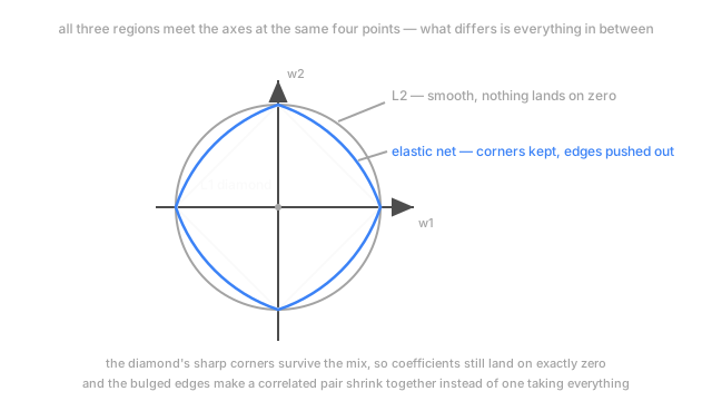
Add even a little of that second term and the flat segment tips into a bowl. Correlated genes shrink toward each other, enter together, leave together. The corners survive, so genes with nothing to contribute still land on exactly zero. That's the shape in the diagram above: corners intact, edges pushed out.

The cap lasso can't lift

With seventy-two rows, lasso returns at most seventy-two nonzero coefficients. Structural, not a tuning artefact. If the pathway holds three hundred genes, lasso can't say so.

The squared term removes that ceiling. It makes the objective strictly convex in every direction, so there's one unique solution and no reason for it to stop at seventy-two. Wide data is where this pays: gene expression, text n-grams where "not worth" and "not worth it" co-occur, one-hot columns off a high-cardinality category. Correlated clusters aren't the exception there, they're the shape of the data.

When not to bother

If your columns are close to independent, stay on pure lasso. Nothing to group, and you keep the sparser model and the smaller grid. If you don't need a shortlist at all, use ridge — it ties elastic net on held-out error more often than people expect, on one dial.

Elastic net earns its second dial in one situation: you need a sparse model and correlated clusters exist. Common enough to matter, rare enough to check.

Show Me the Code

Eight genes instead of twelve thousand. The first four are one co-regulated cluster, each with a true coefficient of 1. The last four are noise.

1import numpy as np2
3
4def enet(X: np.ndarray, y: np.ndarray, lam: float, rho: float, sweeps: int = 2000) -> np.ndarray:5    w = np.zeros(X.shape[1])6    for _ in range(sweeps):7        for j in range(X.shape[1]):8            g = (y - X @ w + X[:, j] * w[j]) @ X[:, j] / len(y)9            t = max(g - lam * rho, 0.0) - max(-g - lam * rho, 0.0)  # the L1 half still clips to 010            w[j] = t / (X[:, j] @ X[:, j] / len(y) + lam * (1.0 - rho))  # L2 half sits below the line11    return w12
13
14rng = np.random.default_rng(5)15X = rng.normal(size=(72, 8))16pathway = rng.normal(size=72)17X[:, :4] = pathway[:, None] + rng.normal(0.0, 0.05, (72, 4))  # four co-regulated genes18y = X[:, :4].sum(axis=1) + rng.normal(0.0, 0.5, 72)19for rho in (1.0, 0.5):20    print(f"rho {rho}:  " + "  ".join(f"{v:+.2f}" for v in enet(X, y, 0.2, rho)))21    # -> rho 1.0:  +0.00  +0.00  +1.40  +2.42  +0.00  +0.00  +0.00  +0.0022    # -> rho 0.5:  +0.92  +0.93  +0.97  +1.00  +0.00  +0.00  +0.00  +0.00

Pure lasso keeps two of the four and loads 2.42 onto a gene that deserves 1.00. Halve the mixing ratio and all four come back between 0.92 and 1.00, the truth, while the noise genes stay at exactly zero. The cluster carries 3.82 either way — only the story about which gene matters changes.

Watch Out For

A grid too coarse to separate the two dials, reported as if the ratio meant something

The symptom: three values of $\rho$ , five of $\lambda$ , a winner at $\rho = 0.5$ , and a line in the write-up about the model needing a balanced mix. Refit on a finer grid and $\rho = 0.9$ wins by less than the fold-to-fold spread. The ratio never meant anything. It was the argmax of noise.

Search $\lambda$ on a log scale and weight the $\rho$ grid toward the high end — 0.5, 0.7, 0.9, 0.95, 0.99, 1 — because behaviour shifts fast near pure lasso and barely at all near pure ridge. Report the fold spread beside the winner; when the top few settings sit inside it, pick the sparsest. Cross-validation schemes covers getting that spread honestly.

Reaching for elastic net when the real problem is unscaled columns

Expression counts in the thousands beside a ratio between 0 and 1, no standardisation, and a penalty that charges the ratio's coefficient ten thousand times more for the same effect. Selection looks unstable, so you add a second penalty and a second dial, and it stays unstable. Both penalties charge by magnitude, and magnitude is set by whoever chose the units.

Standardise every column first, and do it inside each fold or you leak held-out statistics into training. Then refit pure lasso and see whether the instability survived. Often it hasn't. Feature scaling has the mechanics.

The Quick Version

The penalty is $\lambda(\rho \lVert w \rVert_1 + \tfrac{1-\rho}{2}\lVert w \rVert_2^2)$ — one dial for strength, one for the blend, with $\rho = 1$ lasso and $\rho = 0$ ridge.
The grouping effect is why it exists. L1 alone is flat across every split of a correlated pair, so the split lands at an extreme; L2 makes it a parabola whose minimum is the even split.
Correlated features then enter and leave the model together, and the selected set survives a resample.
Corners on the axes survive the mix, so coefficients still reach exactly zero. Sparsity is softened, not traded away.
No cap on how many features get selected, unlike lasso's ceiling of $n$ . That's what makes it usable when features outnumber rows.
The cost is a second hyperparameter. Skip it when columns are near-independent, or when you don't need a shortlist at all.