Core ML

Backpropagation

One forward pass stores what each layer computed. One backward pass hands every parameter its gradient, because the gradients share almost all their work.

Forward values travel left to right and get cached on the way through, then one backward sweep right to left turns the gradient leaving the loss into every parameter gradient in the network

Why Does This Exist?

Training a network needs one number per parameter: how much the loss moves when that parameter moves.

There's an obvious way to get it. Nudge a parameter by a hair, run the network again, see how the loss changed, divide by the nudge. Four lines of code, and one forward pass per parameter. A million parameters, a million passes per step.

Backpropagation gets all million in one backward pass. A step costs around three forward passes, whether the model holds four parameters or seventy billion. At 5 ms a pass, that's ninety minutes against fifteen milliseconds.

Those gradients aren't a million separate problems. They overlap, and the overlap has a shape you can use: the gradient arriving at a layer is exactly what every parameter in that layer needs. Compute it once, let all of them read it, pass a reshaped copy down.

One tiny network carries the page: it predicts how many bikes are still docked at a bike-share station at 6pm from this morning's rainfall. Four parameters, so every number fits on screen.

Two ideas first. A computation graph is the network as a list of small operations with values flowing between them. The chain rule says that if moving $a$ moves $b$ and moving $b$ moves $c$ , then $a$ 's effect on $c$ is the two sensitivities multiplied. Full treatments: computational graphs, the chain rule.

Think of It Like This

Walking a forty-minute delay back down the courier chain

A parcel lands forty minutes late. Four legs got it there: pickup driver, sorting hub, line haul, final van. For each you want one number — minutes saved at the door by making that leg a minute faster. The slow way re-runs the delivery four times. The fast way starts at the door and walks back, each leg needing only the number handed over by the leg after it, times its own local ratio.

The van is minute-for-minute, so its number is 1. This van pulled out half-loaded, so a minute lost on the haul pushed it only half a minute: 1 times 0.5. And the haul waits for a full pallet, so a minute at the hub cost it two: 0.5 times 2, back to 1.

Nobody saw the whole route. And you needed the trip log, because "pulled out half-loaded" is what happened, not what was scheduled.

How It Actually Works

The forward pass, and what it keeps

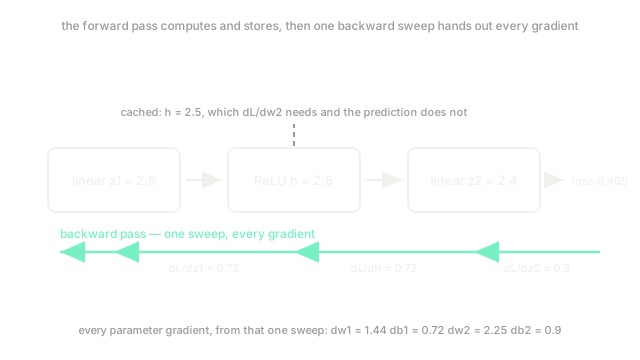
z_1 = w_1 x + b_1, \qquad h = \max(z_1,\, 0), \qquad z_2 = w_2 h + b_2

$w_1$ and $b_1$ are the first layer's weight and bias, $z_1$ the score it produces, $h$ that score with negatives clipped to zero, $w_2, b_2$ the output pair. Set them to 1.5, −0.5, 0.8 and 0.4, then feed in 2 mm of rain.

$z_1 = 2.5$ , positive, so the clip passes it and $h = 2.5$ . Then $z_2 = 2.4$ , a prediction of 24 bikes. Fifteen were there, so squared error puts the loss at 0.405.

Inference stops here and discards both. Training can't: the backward pass needs $h$ 's value and $z_1$ 's sign, so the forward pass caches them.

That's why training and inference memory behave nothing alike. Activation memory scales as depth times batch times width: forty layers emitting 4096-wide vectors at a batch of 256, four bytes a number, is 160 MiB before a single weight. Inference pays none of it.

The backward pass, and the number everything reuses

Start at the loss and ask one thing: how it moves when the output score moves. For squared error that's $z_2 - y = 0.9$ .

Watch how far that 0.9 travels. The output weight's gradient is $0.9 \times h = 2.25$ . The output bias's is $0.9$ . The gradient to send down is $0.9 \times w_2 = 0.72$ . One number, three uses, and the 2.25 is where the cached $h$ gets spent.

Into the clip: $z_1$ was positive, gate open, gradient through untouched at 0.72. Negative and the gate shuts, everything below gets zero — the cached sign earning its keep.

Same move again: the first layer's weight gradient is $0.72 \times x = 1.44$ , its bias gradient $0.72$ .

Four gradients out of two shared numbers. Scale it up and nothing changes in kind: each layer computes one gradient vector, and every parameter in it reads from that.

The output layer used three things — the gradient from above, its own cached input, its own weight. It never learned a clip sat beneath it. Every layer is like that.

That locality is why autograd exists. A framework holds no formula for your network's gradient, just one backward rule per operation composed in reverse order of the forward trace. Which is why a model with a Python if in it still differentiates correctly.

And backpropagation never moves a weight. It hands you four numbers and stops. Step size and direction are gradient descent, and conflating the two is the costliest confusion here.

Show Me the Code

The same network twice: gradients by walking backwards, then the naive way.

1def loss(x: float, y: float, p: list[float]) -> float:2    z1 = p[0] * x + p[1]3    return 0.5 * (p[2] * max(z1, 0.0) + p[3] - y) ** 24
5def backward(x: float, y: float, p: list[float]) -> list[float]:6    z1 = p[0] * x + p[1]7    h = max(z1, 0.0)  # cached, because dL/dw2 needs h and the prediction never reads it again8    g2 = p[2] * h + p[3] - y  # dL/dz2, and all three lines below reuse this one number9    g1 = g2 * p[2] * (1.0 if z1 > 0.0 else 0.0)10    return [g1 * x, g1, g2 * h, g2]11
12P = [1.5, -0.5, 0.8, 0.4]13step = 1e-614print([round(g, 4) for g in backward(2.0, 1.5, P)])15print([round((loss(2.0, 1.5, P[:i] + [P[i] + step] + P[i + 1:]) - loss(2.0, 1.5, P)) / step, 4)16       for i in range(4)])  # one extra forward pass per parameter, which is the whole problem17# -> [1.44, 0.72, 2.25, 0.9]18# -> [1.44, 0.72, 2.25, 0.9]

Identical to four decimals. One version needed a single pass, the other five — fine for four parameters, hopeless for four million.

Watch Out For

Out of memory in training on a model that serves fine

The symptom is specific: the model serves happily at inference, sometimes at a larger batch than you train with, then dies on the first backward call. The forward pass is now holding every hidden activation until the backward pass consumes it, so peak memory jumped by depth times batch times width while the parameter count stayed put.

Two levers. Cut the batch size, since activation memory is linear in it and gradient accumulation recovers the effective batch. Then gradient checkpointing: keep every eighth activation and recompute the seven between.

Debugging the backward pass when the learning rate is the problem

Loss climbs steadily, or hits nan on step 300, and the instinct says the gradients are wrong. So the afternoon goes into gradient checks and hooks printing norms, and nothing moves, because the backward pass was correct all along.

Backpropagation reports slopes. It has no opinion about how far to walk. A diverging loss almost always means the step was too long for the curvature, so the fix lives in the optimiser: lower the learning rate, add warmup, clip the gradient norm.

The Quick Version

One forward pass, one backward pass, every gradient — around three forward passes of work per step, whatever the parameter count.
The saving is reuse: the gradient arriving at a layer is what all of that layer's parameters need, so it gets computed once.
The forward pass caches its activations because the backward pass consumes them. That's why training memory scales with depth and batch size and inference memory doesn't.
Each layer's backward step is local — gradient from above, own cached inputs, own parameters.
Backpropagation computes gradients and updates nothing. The update is gradient descent.
A diverging loss is an optimiser problem far more often than a backward-pass problem.