Core ML

Gradient-Boosted Tree Libraries

Production boosting libraries add three things to the algorithm: features bucketed into bins, the greediest leaf grown first, and categories encoded in order.

Bucketing a feature into a couple of hundred bins once, up front, turns the search for a split from a scan over every row into a scan over bin boundaries

Why Does This Exist?

A motor insurer has four million policies and wants a claim-cost estimate for each before renewal season. Forty features apiece: mileage, years licensed, postcode, last year's premium, and a vehicle-model column holding about 12,000 distinct values.

Gradient boosting already answers the modelling question — fit a small tree to the negative gradient of your loss, shrink it, add it, repeat. Nothing in that recipe is wrong. Implement it as written and you'll be waiting until Thursday.

Where the time goes is what the fix targets. To split one node, a decision tree sorts the rows by a feature and evaluates the gain at every gap between neighbouring values. Four million rows across forty features is 160 million candidate thresholds — for one split. A tree has dozens of nodes, and you wanted a thousand trees.

The vehicle-model column fails differently: one-hot encode it and you've added 12,000 near-empty columns whose best available split isolates a few hundred policies.

So the interesting part of a production library was never the API. It's three ideas, and the third is a statistics fix rather than a speed trick.

Think of It Like This

Grading apples on a slotted board

A packing shed grades apples by weight. The obvious way: line all 40,000 up in weight order and try every dividing point.

The shed builds a board with 256 slots instead, each covering a narrow weight range, and drops every apple through once. Each slot keeps a running count and total. Choosing grade boundaries is now a walk along 255 slot edges, reading two numbers at each. The apples are never sorted again.

What you gave up: you can't cut between two apples that landed in the same slot. Nobody cares, because a slot holds apples within a few grams of each other. And the board gets built before any grading rule exists — pay for that pass once and every later question is cheap.

How It Actually Works

Bucket the feature once, then scan bins

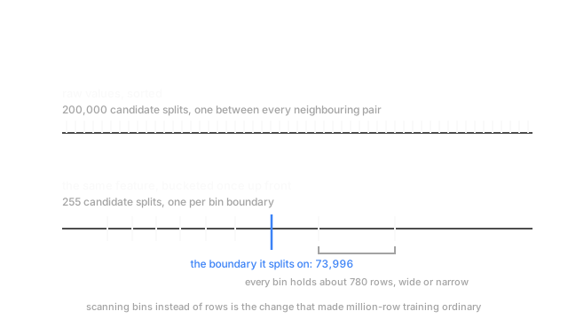
Histogram splitting. Before training starts, each feature is cut into roughly 256 bins, usually at quantiles so every bin holds a similar number of rows. Mileage stops being a float and becomes a bin index that fits in one byte. A node's work is then one pass over its rows to fill the accumulators, then a walk over the boundaries: bins times features, not rows times features.

Two numbers land in each bin. The gradient sum you'd expect, and the sum of second derivatives — the curvature of the loss, how fast the slope itself is changing. With both, a leaf's value comes from a division rather than a fixed step: minus the gradient sum, over the curvature sum plus a penalty. A Newton step per leaf, which is why these libraries need fewer rounds.

Missing values also get a bin of their own, so each split learns which side they belong on. No imputation, no sentinel mileage of minus one.

Grow the greediest leaf, not the level

Textbook trees grow level by level. Leaf-wise growth keeps a queue of candidate leaves scored by the loss reduction each split would deliver, expands the single best one, and repeats until the leaf budget runs out.

For a fixed number of leaves that reaches a lower training loss, since nothing is spent on splits that barely helped. It also overfits faster, and it builds lopsided trees: one branch fourteen deep chasing a few hundred taxi policies while another stops at three.

So the primary control is a cap on total leaves plus a minimum row count per leaf. Depth alone doesn't constrain a tree growing sideways.

Encode a category without leaking the label

Now those 12,000 vehicle models. The natural move is target encoding: replace each model with the average claim cost of the policies carrying it. Compute that average over the whole training set and you've broken the model — each row's own claim cost sat inside the average you handed it, and for a model with three policies, that row is most of its own feature.

Ordered target statistics is the repair. Fix a random permutation of the rows. For each row, compute its category's mean from rows earlier in that permutation only — row 900 sees the 899 before it, never itself. Average across several permutations to steady the early rows, which are noisy because little precedes them.

Same logic as evaluating on data you didn't train on, pushed down into one feature.

Show Me the Code

The binning claim, checked against an exhaustive search on 200,000 odometer readings.

1import numpy as np2
3def best_split(x: np.ndarray, y: np.ndarray, cuts: np.ndarray) -> tuple[float, float]:4    order = np.argsort(x)                            # gain from prefix sums: one pass, any candidate set5    xs, ys = x[order], y[order]6    total, n = ys.sum(), len(ys)7    left_n = np.clip(np.searchsorted(xs, cuts), 1, n - 1)8    left_s = np.cumsum(ys)[left_n - 1]9    gain = left_s ** 2 / left_n + (total - left_s) ** 2 / (n - left_n) - total ** 2 / n10    k = int(np.argmax(gain))11    return float(cuts[k]), float(gain[k])12
13rng = np.random.default_rng(11)14miles = rng.gamma(2.0, 30_000.0, 200_000)            # one policy's odometer reading15cost = (miles > 74_000).astype(float) * 2.0 + rng.normal(0.0, 1.0, 200_000)16exact = np.unique(miles)                             # every gap between two rows is a candidate17bins = np.quantile(miles, np.linspace(0.0, 1.0, 257)[1:-1])18print(f"exact:  {len(exact):>7,} candidates, split at {best_split(miles, cost, exact)[0]:,.0f}")19print(f"binned: {len(bins):>7,} candidates, split at {best_split(miles, cost, bins)[0]:,.0f}")20# -> exact:  200,000 candidates, split at 74,00021# -> binned:     255 candidates, split at 73,996

The break was planted at 74,000 miles. Searching 200,000 candidates finds it; searching 255 lands four miles away, for a tenth of a percent of the work.

Watch Out For

Target-encoding a category over the whole training set

The symptom is loud once you know it. Training error falls through the floor, validation error doesn't move, and the encoded column tops the importance chart. You've built a feature that contains the label.

It bites hardest where target encoding looked most attractive: rare categories. A model with two policies gets an encoding that's essentially the mean of those two labels. Fix it with out-of-fold encoding, or with the ordered scheme above — most libraries will do it for you if you hand them the raw column. Leakage through a hand-built feature is the version no train/test split catches.

Controlling a leaf-wise tree with max depth alone

Set depth to 8, leave the leaf cap at its default, and one branch reaches depth 8 down a narrow path while its siblings stop at 2. Depth 8 permits 256 leaves, most spent on a few hundred rows.

The result looks tuned and generalises unevenly: solid on the bulk of policies, wild on the segments those deep branches describe. Cap the leaf count, and set a minimum rows-per-leaf matching how small a segment you'd trust — a few hundred, not twenty.

The Quick Version

Histogram splitting bins each feature into about 256 buckets once, so split search costs bins times features rather than rows times features.
Each bin carries a gradient sum and a curvature sum, so leaf values come from a Newton step, and missing values get a bin of their own.
Leaf-wise growth expands whichever leaf reduces the loss most: lower training loss per leaf, faster overfitting, lopsided trees. Cap leaves and rows per leaf, not just depth.
Ordered target statistics encode a high-cardinality category from rows earlier in a random permutation, keeping a row's label out of its own feature.
For mixed-type tabular data this family is the default, and two of these libraries differ less than a tuned model differs from an untuned one.