Instrumental Variables (IV)
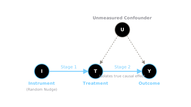
When a confounder completely obscures the causal effect, find a random variable (an instrument) that only affects the treatment, not the outcome. It acts as a natural randomized experiment hidden inside your observational data.
Why Does This Exist?
In observational data, you are plagued by unmeasured confounders (e.g., user motivation, hidden health conditions) that ruin your ability to calculate a true causal effect.
- You can't use Propensity Score Matching, because you don't have the data for the confounder.
- You can't use Difference-in-Differences, because the confounder changes over time.
- You can't run an A/B test, because it's unethical or impossible.
Instrumental Variables (IV) is the ultimate fallback technique. It allows you to calculate a causal effect even when massive, unmeasured confounders are present. It does this by finding a "cheat code" variable—an Instrument—that mimics a randomized experiment.
Think of It Like This
Think of It Like This
Imagine you want to know if going to college (Treatment) increases a person's income (Outcome). You cannot just compare graduates to non-graduates, because the people who go to college are often highly motivated or come from wealthy families (Unmeasured Confounders), which would increase their income anyway.
You can't force people to go to college (no A/B test). But what if there is a random variable that nudges people to go? Suppose you look at distance to the nearest college. People who live very close to a college are slightly more likely to go than people who live 50 miles away. The distance is completely random relative to their innate motivation, and distance doesn't directly increase their future income. By isolating the subset of people who only went to college because they lived close to one, you can measure the true causal effect of the degree. Distance is your Instrument.
How It Actually Works
In causal graph terms, you have an unmeasured confounder creating a backdoor path between Treatment and Outcome : .
An Instrument is a variable that satisfies three strict conditions:
- Relevance: The instrument actually causes (or predicts) the treatment ().
- Exclusion Restriction: The instrument only affects the outcome by going through the treatment. There is no direct path .
- Unconfoundedness: The instrument shares no common causes with the outcome.
If you have a valid instrument, you can use Two-Stage Least Squares (2SLS) to estimate the causal effect.
Two-Stage Least Squares (2SLS)
- Stage 1: Regress the Treatment on the Instrument. This throws away all the variation in the Treatment caused by the unmeasured confounder, keeping only the "clean", randomized variation caused by the instrument.
- Stage 2: Regress the Outcome on the predicted Treatment from Stage 1. This gives you the causal effect.
IV in A/B Testing (Non-Compliance)
IV is heavily used in tech for A/B tests with Non-Compliance. If you randomly assign 1,000 users to receive a new ML feature (the Treatment Group), but only 400 of them actually click the button to turn it on, your A/B test is broken. The users who clicked it are systematically different from the ones who didn't. Here, the random assignment (the Coin Flip) is the Instrument. It doesn't directly improve the user's experience, but it nudges them to use the feature. 2SLS calculates the causal effect for the "Compliers"—the people who used the feature because they were in the treatment group.
Code
Here is a simplified example of Two-Stage Least Squares to solve non-compliance in an A/B test.
import numpy as npimport pandas as pdimport statsmodels.api as sm
np.random.seed(42)N = 10000
# Unmeasured Confounder (Motivation)motivation = np.random.normal(0, 1, N)
# 1. The Instrument (Random Assignment to Treatment Group)# 50/50 chance, completely independent of motivationinstrument_assigned = np.random.binomial(1, 0.5, N)
# 2. The Treatment (Did they actually use the new ML feature?)# Highly motivated people use it anyway. Assigned people get a +30% nudge.prob_use = 0.2 + 0.3 * instrument_assigned + 0.2 * motivationprob_use = np.clip(prob_use, 0, 1)treatment_used = np.random.binomial(1, prob_use)
# 3. The Outcome (Revenue)# True causal effect of the feature is +$50. Motivation also drives revenue.outcome = 100 + 50 * treatment_used + 20 * motivation + np.random.normal(0, 5, N)df = pd.DataFrame({'Z_assigned': instrument_assigned, 'X_used': treatment_used, 'Y_revenue': outcome})
# --- Naive Regression (Wrong) ---X_naive = sm.add_constant(df['X_used'])model_naive = sm.OLS(df['Y_revenue'], X_naive).fit()print(f"Naive Effect: +${model_naive.params['X_used']:.2f}") # -> ~$63 (Overestimates because of motivation)
# --- Two-Stage Least Squares (2SLS) ---# Stage 1: Predict Treatment using the InstrumentX_stage1 = sm.add_constant(df['Z_assigned'])model_stage1 = sm.OLS(df['X_used'], X_stage1).fit()df['X_predicted'] = model_stage1.predict(X_stage1)
# Stage 2: Predict Outcome using the PREDICTED TreatmentX_stage2 = sm.add_constant(df['X_predicted'])model_stage2 = sm.OLS(df['Y_revenue'], X_stage2).fit()print(f"2SLS Causal Effect: +${model_stage2.params['X_predicted']:.2f}")# -> ~$50.08 (Perfectly recovers the true causal effect!)Watch Out For
Weak Instruments.
If your instrument barely affects the treatment (e.g., living close to a college only increases enrollment by 0.01%), it is a "weak instrument". The 2SLS math involves dividing by the correlation between the instrument and the treatment. If that correlation is close to zero, your estimate will blow up, creating massive variance and invalidating your confidence intervals.
Violating the Exclusion Restriction.
This is the hardest assumption to defend because it cannot be proven with data. If your instrument affects the outcome through any path other than the treatment, your estimate is biased. For example, if colleges are built in wealthy neighborhoods, then "distance to college" also correlates with "local job opportunities" (which directly affects income). The instrument is invalid.
The Quick Version
- Instrumental Variables solve the problem of unmeasured confounding when you cannot run a clean A/B test.
- An Instrument is a variable that is randomly distributed, affects the treatment, but does not affect the outcome directly.
- The standard algorithm for calculating the effect is Two-Stage Least Squares (2SLS).
- In tech, IV is primarily used to analyze A/B tests with Non-Compliance, where users don't actually do what their random assignment told them to do.