Core ML

Isolation Forest

Random cuts isolate an odd point in few splits and a typical point in many, so isolation depth becomes the anomaly score, with no distance or density computed.

A far-out point gets separated from everything else by one or two random cuts, while a point in the thick of the cloud needs many cuts before it sits alone in its own region

Why Does This Exist?

Most anomaly detection methods need a notion of distance or density — how far a point sits from its neighbors, how thin the crowd around it is — and both get expensive and unreliable as columns grow, the same curse of dimensionality that makes distance-based clustering struggle in high dimensions. Isolation forest sidesteps the question entirely: instead of measuring how far a point is from anything, it measures how easy the point is to cut away from everything else, using nothing but random splits.

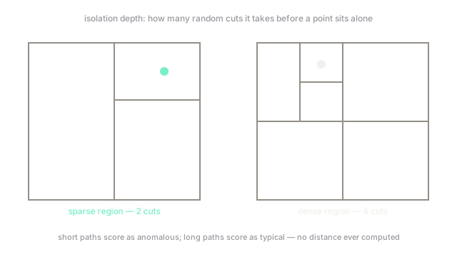
Here's the intuition to carry down the page. A point sitting alone in empty space gets separated from the rest almost immediately by an arbitrary random cut — there's so much empty room around it that nearly any cut isolates it. A point buried in a dense cluster needs many cuts, one after another, before it ends up alone in its own tiny region, since every cut has to fight through the crowd around it first. That difference in how many cuts it takes — the isolation depth — is the entire anomaly score, and it never touches a distance formula.

Think of It Like This

Finding one person in an empty field versus a packed stadium

Someone is hiding in an empty field, and you're trying to find them by drawing random lines across the field and asking "are they on this side or that side" — repeat a couple of times and the field left to search for them is already tiny. Almost any random dividing line isolates them fast, because there was nobody else around to get swept into the same half.

Someone hiding in a packed stadium, playing the same game, doesn't get isolated by two lucky splits. Every line still leaves thousands of others on the same side, and it takes far more splits, cutting the crowd down again and again, before that person is finally alone in a section with nobody else. The field-hider needed almost no work to isolate; the stadium-hider needed a great deal. That difference in effort is isolation depth, and it never required knowing anyone's seat number — only how crowded their neighborhood was.

How It Actually Works

Building one isolation tree

An isolation tree is built the way a decision tree's splits are chosen, except at random rather than by any impurity criterion: at each node, pick a feature and a split value at random, and partition the data into two children. Recurse until every point sits alone in its own leaf, or a maximum depth is reached. No labels are needed and nothing is optimized — the randomness itself is the point, since the tree's structure ends up reflecting only how the data happens to be distributed in space.

The path length for a given point is how many splits it takes, walking down from the root, before that point lands in its own leaf. Points in sparse regions have short path lengths, on average, because random cuts through empty space are likely to separate them quickly. Points buried in dense regions have long path lengths, because most random cuts still leave them bundled with their neighbors.

An ensemble of random trees averages out the luck

A single isolation tree's random splits could get unlucky — a split that happens to isolate a perfectly normal point early, purely by chance. An isolation forest builds many such trees, each with independent random splits, and averages the path length for each point across all of them. Genuine anomalies keep short average path lengths reliably across nearly every tree, since their isolation doesn't depend on any one lucky split. A point that only looked easy to isolate in one unlucky tree gets corrected by the rest of the ensemble.

From average path length to a bounded anomaly score

Average path length alone isn't comparable across datasets of different sizes, so it's normalized against $c(n)$ , the expected path length for a point in a uniformly random dataset of size $n$ — a closed-form quantity from random binary search tree theory. The resulting anomaly score sits in $(0, 1]$ : values near 1 indicate strong anomalies, near 0.5 indicate typical points, and well below 0.5 indicate points the forest struggled to isolate, sitting more centrally than average. This normalization is what lets one numeric threshold work across datasets, rather than needing a size-specific cutoff each time.

Show Me the Code

One obvious outlier, one point sitting in the thick of a normal cloud, scored against a forest trained on the cloud itself.

1import numpy as np2from sklearn.ensemble import IsolationForest3
4rng = np.random.default_rng(3)5normal = rng.normal(0.0, 1.0, (500, 2))6far_anomaly = np.array([[8.0, 8.0]])   # obviously far from the cloud7near_normal = np.array([[0.1, -0.2]])  # sits right in the thick of the cloud8
9x = np.vstack([normal, far_anomaly, near_normal])10forest = IsolationForest(n_estimators=200, random_state=0).fit(x)11scores: np.ndarray = forest.score_samples(x)  # more negative = easier to isolate = more anomalous12
13print(f"typical normal point score:  {scores[:500].mean():.3f}")14print(f"far anomaly score:           {scores[500]:.3f}")15print(f"near-normal point score:     {scores[501]:.3f}")16# -> typical normal point score:  -0.44917# -> far anomaly score:           -0.81718# -> near-normal point score:     -0.388

The far point's score is the most negative of the three — easiest to isolate, shortest average path length — while the near-normal point, sitting closer to the cloud's own center than a typical point, scores even less negative than average. No distance to a centroid or density estimate ever entered the computation; the ordering falls entirely out of how many random cuts each point needed.

Watch Out For

Setting the contamination parameter from a guess rather than domain knowledge

The contamination parameter tells the forest what fraction of the data to expect as anomalous, and it directly sets the decision threshold — a wrong guess doesn't just mislabel a few borderline points, it shifts the cutoff for the whole dataset. A guess pulled from a different population, or a round number like 0.05, can flag several times too many or too few points relative to the real base rate. Estimate it from historical incident rates where they exist, and treat it as a business assumption to validate, not a default to leave alone.

Expecting isolation forest to explain why a point was flagged

An isolation forest's score comes from path lengths averaged over many random trees, and no single feature or split translates cleanly into "this point is anomalous because of column X". Reporting a flagged transaction to a fraud analyst with nothing beyond a score number leaves them unable to act on it. Pair the score with a separate feature-attribution method, such as SHAP, when someone downstream needs a reason rather than just a ranking.

The Quick Version

Isolation forest measures how easy a point is to isolate with random splits, not distance or density to anything.
Path length — how many random cuts isolate a point — is short for anomalies in sparse regions and long for points buried in dense ones.
Averaging path length across many randomized trees corrects for any single tree's lucky or unlucky splits.
The averaged path length is normalized into a bounded score, letting one threshold generalize across differently sized datasets.
The contamination parameter sets the decision threshold directly and should come from real base-rate knowledge, not a default guess.