Core ML

Linear Attention

By replacing the softmax with a kernel function, attention can be rewritten so keys and values are accumulated into a fixed-size running state, making the computation linear in sequence length rather than quadratic.

Why Does This Exist?

Attention complexity establishes that the softmax step forces an $N \times N$ computation: every query scores against every key, giving $O(N^2)$ compute and $O(N^2)$ memory for the score matrix. Sparse attention avoids some cells; FlashAttention tiles them more efficiently. But neither changes the fundamental $O(N^2)$ compute — they reduce constants or memory bandwidth, not the asymptotic cost.

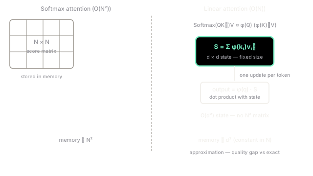
Linear attention is a fundamentally different approach. The idea, going back to Katharopoulos et al. (2020), is to replace the softmax with a kernel function $\phi$ that satisfies a simple decomposition property, then rearrange the order of matrix multiplications. If you can write the attention score as $\phi(q)^\top \phi(k)$ rather than $\exp(qk^\top / \sqrt{d})$ , then the matrix multiplication can be reordered: instead of computing $\text{softmax}(QK^\top) V$ (which needs the full $N \times N$ matrix), compute $\phi(Q)(\phi(K)^\top V)$ , where the inner product $\phi(K)^\top V$ can be accumulated one key-value pair at a time into a $d \times d$ state matrix. Cost drops from $O(N^2 d)$ to $O(N d^2)$ — linear in $N$ .

Think of It Like This

Tallying scores versus computing every pairwise comparison

Imagine ranking 1,000 students by comparing every pair — 500,000 comparisons. Or: compute a feature vector for each student once, then tally how well each student's features match a query profile, by multiplying the query against a running total of feature×score pairs. If the features compose additively, you never need the 500,000-pair table. The tally is a fixed-size intermediate that grows only in feature dimensionality, not in the number of students.

That's linear attention's trick. Instead of materialising all $N^2$ scores, accumulate a running sum of $\phi(k) v^\top$ as each key arrives. When a query comes, dot it against the accumulated state. The state is $d \times d$ , independent of how many tokens have passed.

How It Actually Works

The kernel decomposition

Standard attention:

\text{out}(q_i) = \frac{\sum_j \exp\!\left(\frac{q_i^\top k_j}{\sqrt{d}}\right) v_j}{\sum_j \exp\!\left(\frac{q_i^\top k_j}{\sqrt{d}}\right)}

Linear attention replaces $\exp(q^\top k / \sqrt{d})$ with $\phi(q)^\top \phi(k)$ for some feature map $\phi$ (e.g., elu(x) + 1, or a random Fourier feature approximation). This gives:

\text{out}(q_i) = \frac{\phi(q_i)^\top \sum_j \phi(k_j) v_j^\top}{\phi(q_i)^\top \sum_j \phi(k_j)}

The two sums $S = \sum_j \phi(k_j) v_j^\top$ (a $d \times d$ matrix) and $z = \sum_j \phi(k_j)$ (a $d$ -vector) can be accumulated incrementally. For autoregressive generation, this is exactly a recurrent form: at each new token, update $S$ and $z$ with the new key-value pair, then compute the output with the current query.

The quality gap

The approximation is the price. Softmax has a property called "peakiness" — it concentrates weight on a small number of high-scoring keys. Kernel approximations tend to spread weight more evenly, losing the sharp focus that makes standard attention powerful for tasks that require attending to a specific relevant token. The gap shows up most clearly in retrieval tasks and long documents where finding a specific needle in a haystack matters.

RWKV, Mamba (with its selective SSM), and RetNet all explore different ways to get the speed of the recurrent form while recovering some of the quality.

Show Me the Code

Running a linear-attention pass with the elu + 1 feature map, and checking the output against standard attention.

1import numpy as np2
3rng = np.random.default_rng(3)4n, d = 8, 16   # tiny sequence and head dimension5
6Q = rng.standard_normal((n, d)) * 0.17K = rng.standard_normal((n, d)) * 0.18V = rng.standard_normal((n, d)) * 0.19
10
11def phi(x: np.ndarray) -> np.ndarray:12    """elu(x) + 1 feature map — non-negative, positive-definite kernel."""13    return np.where(x >= 0, x + 1, np.exp(x))14
15
16Qf, Kf = phi(Q), phi(K)17
18# Linear attention output (parallel form, not causal)19S = Kf.T @ V          # (d, d) accumulated KV state20z = Kf.sum(0)          # (d,) accumulated K sum21out_linear = (Qf @ S) / (Qf @ z)[:, None]22
23# Standard softmax attention for comparison24scores = Q @ K.T / d**0.525scores -= scores.max(-1, keepdims=True)26weights = np.exp(scores)27weights /= weights.sum(-1, keepdims=True)28out_softmax = weights @ V29
30diff = np.abs(out_linear - out_softmax).mean()31print(f"Mean absolute difference: {diff:.4f}")32# ~0.05-0.15 — approximation error, not numerical noise

The outputs differ by a measurable amount — the approximation gap in practice. On tasks where sharp focus on a specific key matters, that gap matters too.

Watch Out For

Confusing linear complexity with exact quality

Linear attention is not an efficient implementation of softmax attention. It's a different algorithm with a different (worse) quality profile on many tasks. You don't get the O(N) speed for free — you pay in output accuracy. If your task needs sharp retrieval over long contexts, the quality gap can be the deciding factor.

Assuming the recurrent form and parallel form always give the same answer

In the causal (autoregressive) case, linear attention runs as a recurrence. The parallel training form and the sequential inference form are mathematically equivalent given the same kernel, but small floating-point differences accumulate differently. If your training and inference use different code paths, verify they agree on a small example before trusting the production output.

The Quick Version

Linear attention replaces the softmax with a kernel function $\phi(q)^\top \phi(k)$ , enabling the computation to be rewritten as a running $d \times d$ state matrix rather than an $N \times N$ score matrix.
Complexity drops from $O(N^2 d)$ to $O(N d^2)$ — linear in sequence length.
The recurrent form makes autoregressive inference exactly as fast as processing one token: constant compute per generated token.
The quality gap relative to softmax attention is real and task-dependent; tasks requiring sharp focus on specific keys suffer most.
RWKV and similar architectures build on linear attention's recurrent form while adding selective mechanisms to recover some of the lost quality.