Core ML

Linear Regression

Prediction is a weighted sum plus an intercept, fitted to make the leftover errors smallest. Those leftovers are the most useful thing the model hands back.

The fitted line is the one that makes the total squared length of the vertical residual segments as small as it can be

Why Does This Exist?

A fleet operator retires three hundred delivery vans a year and has to put a reserve price on each before it goes to auction. The obvious lever is the odometer: higher mileage, lower price. So plot price against kilometres for the vans that already sold, draw the line that fits best, and read tomorrow's van off it.

That's linear regression, still the first thing to reach for on a numeric target — not because it's the strongest model but because it tells you things a stronger one won't. One number per feature. The errors it couldn't explain, arranged so you can look at them. And when it's wrong, it's wrong in a nameable shape.

One idea underneath it. A weighted sum takes the numbers about a van — kilometres, age, service visits — multiplies each by its own weight and adds them up. That's the dot product longhand. Add a constant, the intercept, and you have every prediction here.

Think of It Like This

A ruler held by three hundred springs

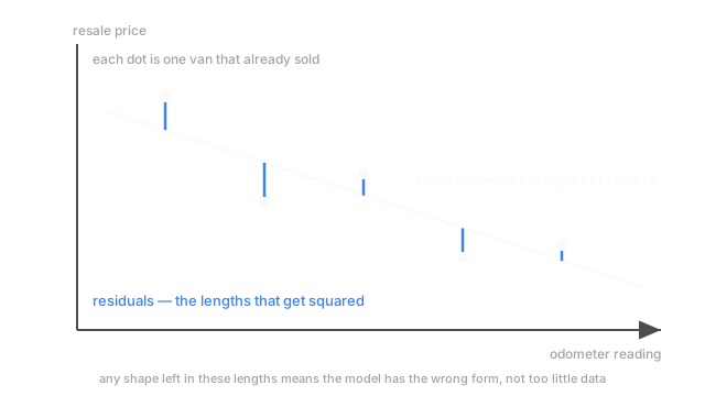
Print the scatter of sold vans on a board, price up, kilometres across. Lay a rigid steel ruler over it, anywhere. Run a spring from each van's dot straight up or down to the ruler — vertical only, never diagonal — and let go.

The ruler tilts and slides and settles. Where it stops is the least-squares fit. Not approximately: exactly. A spring stores energy proportional to the square of its stretch, so the resting position minimises the sum of squared vertical distances, which is the definition of the fit.

That picture pays twice. It shows why vertical distance counts — the springs pull up and down because the errors live in price, not in kilometres. And it shows the weakness. One van that sold for triple what its odometer suggested is a spring stretched three times as far, pulling nine times as hard, and the ruler rotates to appease it.

How It Actually Works

Stack the vans into a matrix $X$ , one row per van, one column per feature, plus a leading column of ones for the intercept, and put the sale prices in a vector $y$ . Every prediction at once is $X w$ , and the fit is whichever weight vector $w$ makes total squared error smallest. It has a closed form:

w = (X^\top X)^{-1} X^\top y

$X^\top$ is $X$ with rows and columns swapped, so $X^\top X$ is square and as wide as you have features. No iteration, no learning rate, no seed — one answer, whenever that product can be inverted. Scale breaks it: fifty thousand one-hot columns makes it a fifty-thousand-square matrix you don't want to build, which is where gradient descent takes over. The geometry behind the formula is ordinary least squares.

What the assumptions buy you

Four get listed, usually without saying what each is for.

Linear in the parameters. Not in the features — in the weights. Squaring kilometres and adding it as a column is still linear regression, and the model can fit a curve. Far weaker than the name suggests.

Independent errors and constant error variance. One van selling above the line should tell you nothing about the next, and the spread should match for cheap vans and expensive ones. Break either and predictions survive while uncertainty estimates go optimistic.

Roughly normal errors. This buys the least and gets quoted the most. Normality makes confidence intervals valid, and says nothing about whether your point predictions are good.

Residuals are the diagnostic

A residual is one van's actual price minus its predicted price: the length of one spring. Plot all three hundred against predicted price and read the shape. Structureless fog is what you want. A smile or a frown means you fitted a straight line to something curved, and depreciation is curved — vans lose value fastest early, so a line overprices the middle and underprices the ends.

Multicollinearity, honestly

Odometer and age correlate at maybe 0.9 in any real fleet. Include both and the coefficients go large and unstable, and refitting on a different year flips the sign on age. Predictions stay fine.

That's not a bug and cleaning data won't fix it. Two near-duplicate columns mean many weight pairs give almost identical predictions, so the fit has no preference and picks on noise. Need stable coefficients? Drop one or shrink with ridge regression.

Show Me the Code

Fit the straight-line version, then the curved one, and measure how much shape is left over.

1import numpy as np2
3rng = np.random.default_rng(1)4km = rng.uniform(10.0, 200.0, 300)  # odometer, thousands of km5price = 34.0 * np.exp(-km / 120.0) + rng.normal(0.0, 0.8, 300)6
7
8def leftover_curvature(design: np.ndarray, y: np.ndarray) -> float:9    w = np.linalg.solve(design.T @ design, design.T @ y)  # solve, never invert10    resid = y - design @ w11    return float(np.corrcoef(resid, design[:, 1] ** 2)[0, 1])12
13
14ones = np.ones_like(km)15for name, design in (("km", np.column_stack([ones, km])),16                     ("km + km^2", np.column_stack([ones, km, km ** 2]))):17    print(f"{name:9s} residual-vs-km^2 correlation {leftover_curvature(design, price):+.3f}")18    # -> km        residual-vs-km^2 correlation +0.19419    # -> km + km^2 residual-vs-km^2 correlation +0.000

The straight-line fit leaves residuals correlated with squared mileage at +0.194. That number is the smile in the residual plot, written as a scalar. Add the squared column and it drops to zero, because the curvature moved out of the leftovers and into the model.

Watch Out For

Reading a coefficient as a cause

The weight on service visits comes out positive: each extra visit predicts a higher price. Somebody writes that up as "servicing a van raises resale value by 400 a visit," and a maintenance budget gets approved on the strength of it.

The coefficient never claimed that. It says that among vans that sold, more service records went with higher prices, holding the other columns where they are. The likely story runs backwards: vans worth keeping got serviced, and vans already written off didn't. If a decision depends on the direction of the arrow, the regression can't settle it.

Trusting R-squared to tell you the model is good

R-squared rises every time you add a column. Every time — including a column of random numbers, which lifts it slightly because the fit can always bend a little toward noise. A report showing 0.94 after twenty features tells you nothing about whether the twenty-first should join them.

Use held-out error instead, in units you can price: regression metrics in currency rather than a ratio. A model at 0.94 that's off by 2,400 on the average van is a worse tool than one at 0.88 off by 900.

The Quick Version

A prediction is a weighted sum of features plus an intercept, fitted by a closed form or by gradient descent when the matrix is too large to factor.
Least squares is the resting position of vertical springs, which is why one outlier moves the line so much.
Linear means linear in the weights. Squared and interaction features are still linear regression.
Normality of errors buys valid confidence intervals, not better predictions.
Residuals against fitted values earns its keep as a diagnostic. Visible shape means the wrong model form.
Correlated features destabilise coefficients while leaving predictions intact.
R-squared only goes up. Judge on held-out error.