Core ML

Matrix Factorization

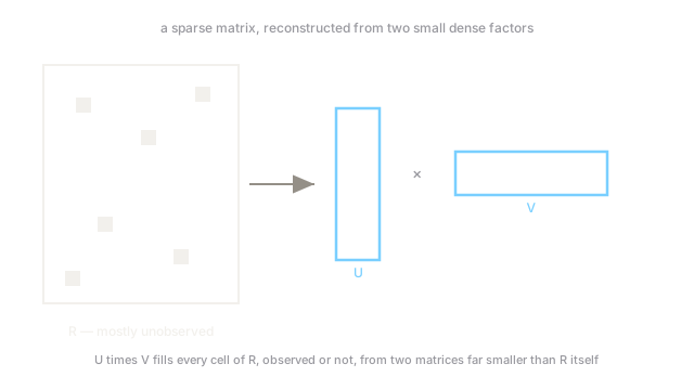
Reconstruct a matrix as the product of two smaller ones, and missing entries fill in for free, since the two factors were fit to explain only entries you have.

A sparsely filled ratings matrix is reconstructed as the product of two much smaller factor matrices, and the product fills in every entry the original matrix never observed

Why Does This Exist?

A streaming service has 40,000 users and 30,000 titles, and any one user has rated maybe a few dozen of them — the ratings matrix is enormous and almost entirely empty. You want to predict what a user would rate the titles they haven't touched, using nothing but the sparse, scattered ratings everyone else left behind.

PCA and the SVD it relies on both assume you can see the whole matrix. Neither has an answer for "most of this matrix was never observed" — SVD's standard algorithm doesn't run on a matrix with holes in it at all. Matrix factorization is the version of "represent this matrix with two much smaller ones" built specifically for the case where most entries are missing, and where filling in those missing entries well is the entire point.

Think of It Like This

Guessing a taste from a handful of dishes tried

A food-delivery app knows, for each customer, a scattered handful of dishes they've rated out of thousands on the menu — nobody has tried more than a sliver of it. You want to guess how a customer would rate a dish they've never ordered.

The trick is to describe every customer by a short list of taste preferences — how much they like spice, how much they like sweetness, how much they favor a particular cuisine — and describe every dish by how much of each of those qualities it has. A customer's predicted rating for any dish, tried or not, is just how well their taste profile matches that dish's profile. You never needed the customer to have tried the dish: you only needed enough of their other ratings to guess their taste profile in the first place, and once you have that, every untried dish gets a prediction for free.

Those taste-profile numbers are exactly what matrix factorization calls latent factors — dimensions nobody labeled in advance, discovered purely from which ratings existed.

How It Actually Works

Splitting one large sparse matrix into two small dense ones

The ratings matrix $R$ , $m$ users by $n$ items, is approximated as the product of two much smaller matrices: a user-factor matrix $U$ ( $m$ by $k$ ) and an item-factor matrix $V$ ( $n$ by $k$ ), where $k$ — the number of latent factors — is far smaller than either $m$ or $n$ . Row $i$ of $U$ is user $i$ 's taste profile; row $j$ of $V$ is item $j$ 's profile, and the predicted rating for any user-item pair is simply the dot product of the two rows, $U_i \cdot V_j$ . Both matrices together hold vastly fewer numbers than the original matrix has entries, which is the compression this method is named for — and the dot product is defined for every user-item pair, filled in or not.

Fitting only on what was actually observed

The factors are found by minimizing squared error, but summed only over the entries that were actually observed — every unobserved cell contributes nothing to the loss and gets no direct gradient signal at all:

\min_{U, V} \sum_{(i,j) \in \text{observed}} \left(R_{ij} - U_i \cdot V_j\right)^2 + \lambda\left(\lVert U \rVert^2 + \lVert V \rVert^2\right)

The regularization term keeps the factors from growing unboundedly to fit noise in a small observed set. Once $U$ and $V$ are fit, the missing entries are never estimated directly — they simply inherit whatever value $U_i \cdot V_j$ produces, because that product exists for every pair regardless of whether it was in the training sum. This is optimized either by gradient descent directly on both matrices at once, or by alternating least squares — fix $V$ , solve for $U$ in closed form, fix the new $U$ , solve for $V$ , repeat — which turns a nonconvex joint problem into a sequence of easy convex ones.

The relationship to PCA and SVD, and where it diverges

Fit matrix factorization on a fully observed matrix with no regularization and it converges toward the same low-rank structure the SVD gives you directly — this is genuinely SVD's generalization to the missing-data case, not an unrelated method that happens to look similar. The divergence is entirely about what each one can handle: SVD needs every entry and gives you the exactly optimal low-rank approximation in one shot; matrix factorization tolerates enormous sparsity and reaches its answer iteratively, trading a guarantee of exact optimality for the ability to run on data SVD structurally can't touch.

Show Me the Code

A synthetic ratings matrix, 70% of entries hidden from training, factored with alternating gradient updates.

1import numpy as np2
3rng = np.random.default_rng(0)4n_users, n_items, rank = 40, 30, 35true_u = rng.normal(size=(n_users, rank))6true_v = rng.normal(size=(n_items, rank))7ratings = true_u @ true_v.T + rng.normal(0.0, 0.1, (n_users, n_items))8
9observed = rng.random((n_users, n_items)) < 0.3  # only 30% of ratings are ever seen10u: np.ndarray = rng.normal(scale=0.1, size=(n_users, rank))11v: np.ndarray = rng.normal(scale=0.1, size=(n_items, rank))12lr, reg = 0.005, 0.0213
14for _ in range(500):15    error = np.where(observed, ratings - u @ v.T, 0.0)  # zero on unobserved entries -- no gradient from them16    u += lr * (error @ v - reg * u)17    v += lr * (error.T @ u - reg * v)18
19held_out = ~observed20rmse = float(np.sqrt(np.mean((ratings[held_out] - (u @ v.T)[held_out]) ** 2)))21print(f"RMSE on held-out (never-seen) ratings after 500 epochs: {rmse:.3f}")22print(f"training used only {observed.mean():.0%} of the ratings matrix")23# -> RMSE on held-out (never-seen) ratings after 500 epochs: 0.32324# -> training used only 32% of the ratings matrix

Trained on 32% of the entries, with zero gradient contribution from the rest, the factorization still predicts the 68% it never saw to within 0.32 of the true rating — the two small factor matrices generalized past what they were shown, because the true structure was low-rank to begin with.

Watch Out For

Choosing rank by fit quality on the observed entries alone

Raising $k$ always improves the fit on entries the model was trained on, the same way adding a tree helps random forests fit training data, and past a point it starts memorizing the specific observed ratings rather than the general taste structure behind them. Choose rank the way any other hyperparameter is chosen — score held-out entries deliberately withheld from fitting, not the training entries the loss was computed on.

Treating a new user's or item's cold-start prediction as meaningful

A user with zero observed ratings has no row in $U$ that was ever fit to anything, so a factorization model has nothing informative to predict for them — a default row will produce some number, but it reflects nothing about that user's actual preferences. This is the cold-start problem, structural to the method rather than a bug: matrix factorization only knows what it was shown, and a user or item outside the training matrix was shown nothing.

The Quick Version

Matrix factorization approximates a large, sparse matrix as the product of two much smaller factor matrices, fit only on the entries that were actually observed.
Missing entries are never predicted directly; they inherit whatever value the factor product happens to produce for that pair.
On a fully observed matrix, it converges toward the same structure the SVD provides directly — this generalizes SVD to handle missing data, at the cost of an exact optimality guarantee.
Alternating least squares turns the nonconvex joint fitting problem into a sequence of easy convex ones by fixing one factor matrix at a time.
New users or items with no observed entries have nothing informative in their factor row — the cold-start problem is structural, not a tuning issue.