Core ML

Ordinary Least Squares

Least squares drops a perpendicular from your data onto everything your features can build. One picture that explains the algebra and where it stops holding.

The fitted values are the orthogonal projection of y onto the column space of X, so the residual leaves that plane at a right angle

Why Does This Exist?

Linear regression hands you a formula for the weights and moves on. Two questions get skipped: why that formula, and why no serious library computes it that way.

Both answers come out of one picture. A greenhouse logs its water use for three days alongside the sunlight hours each day got, so two columns go into the fit: a column of ones, and sunlight hours.

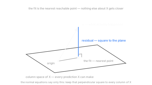
Now the shift that makes everything follow. A list of three numbers is a point in three-dimensional space, so your water readings are one specific point out there, call it $y$ . Your two columns are two other points, which you may scale and add — and every combination sweeps out a flat plane through the origin. That plane is the column space of $X$ : every prediction your features can ever make, everything else unreachable (vector spaces and rank generalises it).

So your data is a point, your reachable predictions are a plane, and $y$ is not on it. Find the closest point on the plane.

Think of It Like This

The shortest string from a fly to the windowpane

A fly hovers a hand's width off a window. Run a string from the fly to any point on the glass and measure it. Slide the far end around: the string shortens, bottoms out, lengthens again.

Look at where the shortest one lands. It meets the glass square on, at a right angle — and nobody imposed that. It falls out of being shortest. Tilt the string a few degrees off perpendicular and you've bolted a sideways leg onto a right triangle, so by Pythagoras it's longer. The perpendicular wins because every other string is a hypotenuse.

That's least squares in full. The glass is every prediction your features can produce, the fly is what happened, the fit is the nearest point on the glass, and the string is the error left over.

How It Actually Works

Write $\hat{y} = Xw$ for the fitted values and $r = y - \hat{y}$ for the residual. Whatever $w$ you pick, $\hat{y}$ lands on the plane. Making $r$ as short as possible means making it perpendicular to the plane, and a vector is perpendicular to a plane exactly when it's perpendicular to everything spanning it — so to every column of $X$ :

X^\top (y - Xw) = 0 \quad \Longrightarrow \quad X^\top X w = X^\top y

Those are the normal equations, where "normal" means perpendicular — nothing to do with the normal distribution. The condition is a list of dot products, one per column, each required to be zero.

One consequence you can check by hand

The intercept column is all ones, and its dot product with the residual is the sum of the residuals. So residuals sum to exactly zero whenever the model has an intercept. Duplicate columns fall out of the same picture: two identical columns don't buy a second dimension, so the plane stays a line and $X^\top X$ can't be inverted. The nearest point is still one point, but the weights reaching it are not unique — decided by matrix rank.

Squared error is an assumption about noise

Squared error looks like the default. It's a claim.

Suppose each day's water use is the true linear value plus independent noise from a bell curve of the same width every day. The probability of your three readings, as a function of $w$ , is a product of those densities, and its logarithm is a sum of squared gaps between observed and predicted. Maximising that log is minimising squared error. Same problem. So squared loss is maximum likelihood under Gaussian noise of constant variance, and heavy tails would make absolute error the likelihood-maximising choice instead. You weren't being neutral. You were assuming.

Why nobody forms the normal equations

The condition number of a matrix measures how much it amplifies small relative errors, so a large one means digits get eaten during the solve. Forming $X^\top X$ squares it: a design matrix at a condition number of a million becomes a system at a trillion, and double precision carries roughly sixteen digits, so you've spent twelve before the solver starts. QR and SVD work on $X$ directly and never form that product, paying the condition number once rather than twice. That's why numpy.linalg.lstsq and R's lm factor instead of using the formula everyone learns.

Show Me the Code

Both claims at once: the residual is orthogonal to every column, and the conditioning squares.

1import numpy as np2
3rng = np.random.default_rng(2)4sun = np.linspace(4.0, 11.0, 60)  # daily sunlight hours5X = np.vander(sun, 8)  # powers of one column, so the columns nearly coincide6water = 120.0 + 18.0 * sun + rng.normal(0.0, 2.0, 60)7
8normal_eq = np.linalg.solve(X.T @ X, X.T @ water)  # forming X'X squares the conditioning9factored, *_ = np.linalg.lstsq(X, water, rcond=None)  # what a library reaches for instead10
11resid = water - X @ factored12cosines = (X.T @ resid) / (np.linalg.norm(X, axis=0) * np.linalg.norm(resid))13print(f"worst angle cosine, residual vs a column: {np.abs(cosines).max():.1e}")14print(f"cond(X) {np.linalg.cond(X):.1e}   cond(X'X) {np.linalg.cond(X.T @ X):.1e}")15print(f"the two coefficient vectors differ by {np.abs(normal_eq - factored).max():.1e}")16print(f"their predictions differ by only     {np.abs(X @ (normal_eq - factored)).max():.1e}")17# -> worst angle cosine, residual vs a column: 4.2e-1118# -> cond(X) 1.3e+11   cond(X'X) 1.8e+2219# -> the two coefficient vectors differ by 1.1e-0120# -> their predictions differ by only     3.1e-05

The cosines come back at 4.2e-11, zero in floating point: the string really is square to the glass. Then conditioning goes from 1.3e+11 to 1.8e+22, past what double precision can represent, so the normal-equations route is hopeless while the factorisation is fine. Their predictions agree to five decimals while their coefficients disagree in the first. The plane is pinned down; the way you describe it isn't.

Watch Out For

Solving the normal equations on data you never conditioned

The symptom is coefficients that swing between runs, or a solver that reports success and returns weights of magnitude ten to the ninth on data measured in litres. Raw polynomial features do it, as does mixing a column in metres with one in nanoseconds. The formula still evaluates. It answers a question a long way from yours.

Use np.linalg.lstsq or a QR solve rather than solve on the cross-product, and centre and scale columns first. Then check the condition number of $X$ : past about ten to the eighth, treat individual coefficients as unreadable whatever solver you used, and either drop columns or move to ridge regression.

Quoting Gauss-Markov as if it said OLS is best

The theorem is real and narrower than its reputation. Under uncorrelated errors of equal variance, OLS has the smallest variance among linear unbiased estimators. Three qualifiers, all load-bearing.

Drop unbiasedness and biased estimators routinely win on held-out error, which is the whole argument for ridge and lasso. And equal, uncorrelated errors is what fails most often: time-ordered data has correlated errors, spend data has variance growing with the level. Both break the guarantee while the arithmetic keeps working, so nothing complains. Check residuals for correlation and a widening fan.

The Quick Version

The fitted values are the orthogonal projection of the target onto the column space of the design matrix, and the residual leaves at a right angle.
The normal equations say one thing: make the residual perpendicular to every column.
With an intercept column of ones, residuals sum to exactly zero.
The projection is always unique. The coefficients producing it are unique only when the columns are independent.
Minimising squared error is maximum likelihood under Gaussian errors of constant variance, so the loss encodes a noise assumption.
Forming the normal equations squares the condition number. QR or SVD pays it once.
Gauss-Markov gives best linear unbiased, which evaporates under unequal or correlated errors.