Core ML

Policy Gradient Methods

Push up the probability of actions that paid off. The estimate is unbiased and wildly noisy, so every refinement after REINFORCE is about shrinking variance.

One update shifts the policy's whole distribution over actions toward a sampled action whose return came back above average, so the policy is nudged rather than told what the right action was

Why Does This Exist?

A robotic arm on a parcel sorting line picks up boxes arriving at a slightly different angle every time. Its actions are real numbers — wrist angle in degrees, gripper force in newtons, descent speed. No list of options to score.

Q-learning needs that list, because taking a maximum means enumerating. Ten buckets of wrist angle throws away the precision that makes a grasp hold. A thousand, times two more dimensions, and the count passes a billion.

Second reason: sometimes the best behaviour is genuinely random. With a parcel's pose only roughly known, a controller that always tries the identical grip either always succeeds on that box shape or always fails.

So stop learning what actions are worth. Optimise the policy itself.

Think of It Like This

The kitchen that grades every dish by the night's total takings

A kitchen tries slight variations each service — more acid in the dressing, thirty seconds less on the fish. At the end of the night, one number: total takings.

Every dish shares it. The best dessert anyone ate all week gets marked down because the kitchen ran out of fish at eight; a mediocre plate on a full Saturday gets a gold star. The signal is real, just buried.

Then someone judges tonight against a normal Tuesday instead of zero. Same information, but the number now means "better or worse than usual". The noise drowning everything was a constant nobody needed.

How It Actually Works

Score the action, then push its probability

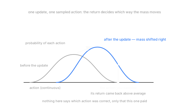
The policy is a network: state in, parameters of a distribution over actions out. For continuous control that's usually a mean and a spread per dimension, so wrist angle is drawn from a bell centred wherever the network thinks it belongs. Exploration comes free, and the policy can narrow that spread itself.

You maximise expected return $J(\theta)$ , with $\theta$ the network's weights. The policy gradient theorem says the gradient of that return is an average over behaviour the policy actually produced:

\nabla_{\theta} J(\theta) = \mathbb{E}\big[\nabla_{\theta} \log \pi_{\theta}(a \mid s)\, G\big]

$\pi_{\theta}(a \mid s)$ is the density the policy puts on action $a$ in state $s$ , $\nabla_{\theta} \log \pi_{\theta}$ is the direction in weight space that makes it more likely, and $G$ is the discounted return that followed. REINFORCE is that expression, sampled.

Notice what's absent — nothing differentiates through the conveyor. You need only your own network's gradient, which is why this works on black boxes and real hardware.

The wall: an unbiased estimate you can't use

It's unbiased, and it converges given enough episodes. The trouble is how many "enough" is.

One sorting cycle is forty actions and one return, and all forty get multiplied by the same number. A textbook grasp in a cycle where the conveyor jammed downstream gets a negative weight and is trained away; a sloppy grasp on a lucky cycle gets reinforced.

Scale makes it worse. Say a cycle earns between 190 and 210. Every action gets multiplied by roughly 200, a constant that says nothing about any individual action while inflating every sample's variance. Monte Carlo estimation has a fixed rate — halve the noise, quadruple the samples. Here, samples are grasps.

Baselines, critics, and a leash on the update

Everything after REINFORCE is variance reduction wearing a different hat.

A baseline subtracts $b(s)$ , anything that depends on the state but not the action. The expectation doesn't move: the expected value of $\nabla_{\theta} \log \pi_{\theta}$ under the policy's own actions is zero, so an action-independent factor vanishes in the average. Variance falls hard.

The natural $b(s)$ is the state value $V(s)$ , what you'd normally get from here. Then $G - V(s)$ is the advantage: how much better this action turned out than usual. Absolute number becomes comparison, the same move the kitchen made. Actor-critic learns $V(s)$ with a second network while the policy trains.

A large update also changes the data you collect next, so an over-eager step can leave the policy gathering useless experience. PPO limits the move bluntly: take the ratio of new to old probability for an action, and stop granting credit once it leaves a narrow band around one.

The bill is sample efficiency: that expectation is over the current policy, so one step leaves your data describing a policy that no longer exists. Q-learning replays a transition dozens of times; this spends a batch once. Sorting arms learn in simulation for a reason.

Show Me the Code

A one-step policy whose return carries a large constant offset.

1import numpy as np2
3
4def grad_samples(baseline: float, trials: int = 20_000) -> np.ndarray:5    """One-step Gaussian policy at mean 0.5; the return peaks at 2.0, plus a flat offset."""6    rng = np.random.default_rng(3)7    a = rng.normal(0.5, 1.0, trials)8    returns = 40.0 - (a - 2.0) ** 2  # the offset is the point: it carries no information9    score = a - 0.5  # gradient of the log density with respect to the mean10    return score * (returns - baseline)11
12
13average_return = 40.0 - (0.5 - 2.0) ** 2 - 1.0  # what this policy earns on average14for b, name in ((0.0, "no baseline"), (average_return, "mean baseline")):15    s = grad_samples(b)16    print(f"{name:14s} mean {s.mean():+.3f}   spread {s.std():7.3f}")17    # -> no baseline    mean +3.118   spread  35.04818    # -> mean baseline  mean +2.968   spread   5.199

The true gradient is exactly 3.0 and both estimates sit near it — unbiased, as promised. The spread drops from 35.0 to 5.2, a factor of seven, purely from subtracting a number that says nothing about the action taken.

Watch Out For

Raw episode returns, and a learning curve that's mostly luck

The return curve climbs, dives, then climbs higher than before. Re-run with a different seed and the shape is unrecognisable — two seeds look like two algorithms, and you can't tell whether last week's change helped.

That's REINFORCE with no baseline. Variance is large enough that which episodes went well dominates which actions were good, so training follows the sampling noise. Keep a running average of recent returns and subtract it; the curves tighten immediately. Then move to a state-dependent baseline, because one scalar can't separate a hard state from a badly chosen action.

Bolting a replay buffer onto an on-policy method

Value learning got dozens of updates per transition, so the temptation is obvious: keep the last hundred thousand grasps and sample from them. Throughput looks great, then the policy quietly gets worse while the loss stays healthy.

The expectation is over actions the current policy would take. Data from three updates ago came from a different distribution, so averaging it in estimates the gradient of a policy you no longer have — biased, not just noisy, and more data doesn't fix bias. Correct it with an importance ratio between new and old policy, which is what PPO's clipping keeps from exploding, or just collect fresh batches.

The Quick Version

A network outputs a distribution over actions; you do gradient ascent on expected return. Continuous actions need no discretisation.
The gradient is the log-probability gradient of the action taken, weighted by the return that followed. REINFORCE is that, sampled.
Nothing differentiates through the environment.
Unbiased, and brutally noisy: one return is shared across every action in the episode, so good actions in bad episodes get punished.
A baseline cuts variance sharply. Set it to $V(s)$ for the advantage; learn it with a second network for actor-critic.
Limit each update, because it changes the data you collect next. PPO clips the probability ratio.
On-policy, so data goes stale every step — orders of magnitude more interaction than off-policy value learning.