Policy Gradient Theorem

You can improve a policy without modeling the world by following the gradient of expected reward, estimated from the rewards your own actions actually earned.

Two sampled trajectories earn different returns, and the policy shifts toward the actions of the higher earning run

Why Does This Exist?

Value methods learn by bootstrapping predictions of future reward, which breaks when function approximation distorts those predictions. Policy methods skip the middleman: they tune the action probabilities directly to earn more. But differentiating expected reward looks impossible at first, because the expectation depends on unknown transition dynamics.

The policy gradient theorem removes the dynamics from the derivative. It shows the gradient depends only on the policy's own score function and the returns actually observed, so sampling episodes suffices. REINFORCE, actor-critic, and PPO all rest on this identity. This page proves the shape and shows the variance fix.

The one idea you need first

The score function is $\nabla_\theta \log \pi_\theta(a|s)$ : how a parameter nudge changes the log probability of an action. Its expectation under the policy is zero, which is why it can weight returns without bias. Expectation, variance and covariance cover the averaging rules used below.

Think of It Like This

Tipping restaurant dishes by profit

You run a food stall with three dishes and want more profit. Each day you note which dishes customers picked and the day's takings. To adjust the menu, you push probability toward dishes sold on high-profit days and away from dishes sold on losing days, scaled by how surprising each sale was.

Returns are the daily takings, the score function is the surprise adjustment, and the policy is the menu mix. Where the analogy stops: real menus change customer arrivals (the dynamics), but the theorem shows you never need that arrival model to compute the direction.

How It Actually Works

For episodic return $G_t$ and parameters $\theta$ , the theorem states:

\nabla_\theta J(\theta) = \mathbb{E}_\pi\left[ G_t \, \nabla_\theta \log \pi_\theta(A_t|S_t) \right]

In plain words: weight each action's score direction by the return that followed it, then average over experience. High-return actions get reinforced along their score vector; low-return actions get pushed away. The environment dynamics $P(s'|s,a)$ never appear because differentiating the log probability cancels them through the likelihood-ratio trick.

REINFORCE samples this directly: run an episode, and for each step add $G_t \nabla \log \pi$ . Variance is brutal, so actor-critic subtracts a baseline $b(S_t)$ , usually the value estimate, without bias:

\nabla J = \mathbb{E}[ (G_t - b(S_t)) \nabla \log \pi ]

Worked example

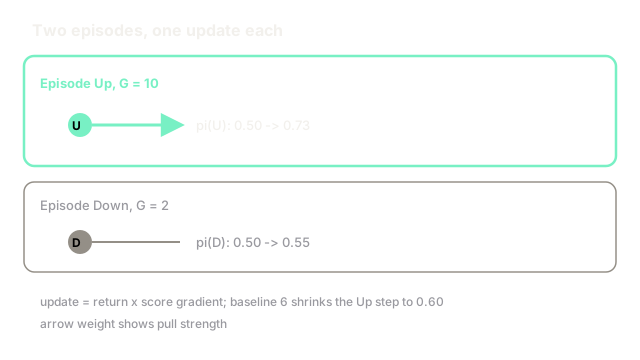
One state, two actions with logits $\theta = [0, 0]$ , so $\pi = [0.5, 0.5]$ . Action Up always returns $G = 10$ , Down returns $G = 2$ . Sample Up once.

Score for Up under softmax: $\nabla \log \pi(U) = [1 - 0.5, -0.5] = [0.5, -0.5]$ . REINFORCE step with rate $0.1$ : $\Delta = 0.1 \times 10 \times [0.5, -0.5] = [0.5, -0.5]$ . New logits $[0.5, -0.5]$ give $\pi(U) = e^{0.5}/(e^{0.5} + e^{-0.5}) \approx 0.731$ . One good episode moved Up from 50 to 73 percent. With baseline $b = 6$ (mean return), the weight drops to $10 - 6 = 4$ and the step lands at $\pi(U) \approx 0.599$ , smaller and steadier.

Code

1import numpy as np2
3
4def softmax(z: np.ndarray) -> np.ndarray:5    e = np.exp(z - z.max())6    return e / e.sum()7
8
9theta = np.array([0.0, 0.0])10p = softmax(theta)  # [0.5, 0.5]11score_up = np.array([1 - p[0], -p[1]])  # grad log pi(Up)12theta_new = theta + 0.1 * 10.0 * score_up  # REINFORCE, G=1013print(softmax(theta_new))  # -> [0.73105858 0.26894142]

The printed probabilities match the hand step: 0.731 for Up after one reinforced episode.

Watch Out For

Forgetting the baseline must not depend on the action

A baseline that uses the sampled action, like the return of a different action in the same state, leaks bias into the gradient. The proof needs $b$ to depend on state only so its score-weighted expectation stays zero. Action-dependent bonuses silently tilt the policy.

Use $V(s)$ or a running average of returns, never the advantage of a cherry-picked action.

Sampling with too large a step

Policy gradients are noisy, and a step of 0.1 on a 10-return signal moves probabilities by 20 points, as the example shows. Two such steps in a row can collapse exploration to a near-deterministic policy before values are known. Loss looks great while evaluation on new starts fails.

Keep steps small, clip updates as PPO does, or normalize returns per batch. If entropy collapses in the first hundred episodes, the rate is the suspect.

The Quick Version

The policy gradient is expected return times the score function, with no dynamics model needed.
REINFORCE samples it from complete episodes; actor-critic subtracts a state baseline to cut variance.
The one-state example moves Up from 0.50 to 0.73 on a single return of 10.
Baselines must depend on state only, or bias creeps in.
Small steps or clipping protect against premature entropy collapse.