Core ML

Pooling Layers

Shrink a feature map by keeping only the strongest signal in each small patch, trading exact position for tolerance to roughly where a pattern sat.

Shifting a strong signal to a different cell within the same pooling window still reports the same maximum, which is where pooling's tolerance to position comes from — and where it runs out

Why Does This Exist?

Train a network to recognize a cat photographed slightly left of center, then show it the same cat one inch to the right, and a network built purely from convolutions treats that as a materially different input. The whisker-detecting kernel fires at a different pixel location, and every layer downstream inherits that shift. Nothing forces the network to treat "cat, shifted an inch" as the same fact as "cat".

There's a second, more practical wall. A photo entering the network at 224×224 stays roughly that size through several convolutional layers — padding keeps the spatial dimensions from shrinking too fast — so the feature maps stay large, and large feature maps mean every downstream layer, and the classifier at the very end, is expensive.

Pooling attacks both problems with one operation: look at a small patch of the feature map, keep a single summary number, and throw the rest away. Do that everywhere, and the map shrinks and small shifts inside each patch stop being visible at all.

Think of It Like This

A show of hands instead of a headcount

Ask a packed room "does anyone here know the answer?" and you don't need a precise count of every hand — you need one bit: did anyone raise a hand at all. If three people near the front raise their hands versus three people near the back, the room's answer is identical: yes.

Max pooling asks that question of a small patch of a feature map. It doesn't care exactly where in the patch the loudest signal was — only that it was there, and how strong. Move the strongest hand-raiser one seat over, and as long as they're still in the same section of the room, the room's answer doesn't change.

How It Actually Works

Max pooling, the default

Slide a small window — 2×2 is the most common size — across the feature map, and at each position keep only the single largest value inside it. Unlike a convolution kernel, there are no learned weights here: the operation is fixed, just "take the maximum."

A 2×2 window with stride 2 (matching the window size, so patches never overlap) halves both the height and width of the map. A 224×224 feature map becomes 112×112 after one such layer — a quarter of the values survive, and they're the strongest quarter, not an arbitrary one.

Where the invariance comes from, and where it stops

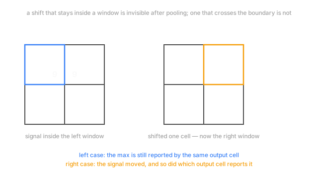
The diagram above shows the exact mechanism. A strong signal sitting anywhere inside one 2×2 window produces the same output for that window, regardless of which of the four cells it's actually in — the max of {9, low, low, low} is 9 no matter which corner the 9 occupies. That's the "tolerance to roughly where a pattern sat" from this page's intuition, made concrete: small, sub-window shifts genuinely vanish.

Shift the signal one cell further, so it crosses into the next window, and the invariance breaks immediately — a different output cell now reports the maximum, and the one that used to report it drops back to whatever else was in its window. Pooling doesn't grant true position invariance; it grants invariance in patches equal to the window size, and nothing beyond that. Stack several pooling layers and the tolerance compounds, because each one is working on a map already shrunk by the last — which is also exactly how receptive fields grow with depth.

Average pooling, and why max usually wins for detection

Average pooling replaces "take the max" with "take the mean" over the same window. It's smoother — no single pixel can dominate the output — which made it common in early architectures. For detecting whether a specific pattern is present, though, averaging is the wrong instinct: a strong, sharp activation exactly where an edge or a texture fired gets diluted by every quiet neighboring cell in the same window. Max pooling preserves the strongest response instead of blending it away, which is why it became the default for classification stacks.

Average pooling still earns a specific job: global average pooling, which averages an entire feature map — not a small window, the whole thing — down to a single number per channel, right before the final classification layer. That single design choice is what lets a network accept images of different sizes: whatever the feature map's spatial dimensions happen to be, averaging collapses them to one number per channel, and the classifier only ever sees a fixed-length vector.

The alternative that's slowly replacing it

Some modern architectures drop pooling for spatial downsampling entirely and use a strided convolution instead — a convolution with stride greater than 1, so it both extracts features and shrinks the map in the same operation, with learned weights doing the summarizing instead of a fixed max or average. Pooling remains far more common in practice, particularly global average pooling at the head of a network, but "convolution with a stride" is worth recognizing as the same job done a different way.

Show Me the Code

Max pooling and average pooling over the same 4×4 input, computed with plain loops so the window-by-window mechanism stays visible.

1import numpy as np2
3
4def pool2x2(x: np.ndarray, mode: str = "max") -> np.ndarray:5    oh, ow = x.shape[0] // 2, x.shape[1] // 2  # 2x2 windows, stride 2 -> halves each dim6    out = np.zeros((oh, ow))7    for i in range(oh):8        for j in range(ow):9            window = x[i * 2 : i * 2 + 2, j * 2 : j * 2 + 2]10            out[i, j] = window.max() if mode == "max" else window.mean()11    return out12
13
14feature_map = np.array([[1, 1, 0, 0], [1, 9, 0, 0],15                         [0, 0, 1, 1], [0, 0, 1, 1]], dtype=float)16
17print(pool2x2(feature_map, "max"))18# -> [[9. 0.]19#     [0. 1.]]20print(pool2x2(feature_map, "average"))21# -> [[3.   0.  ]22#     [0.   1.  ]]

Max pooling reports the 9 untouched — it survives the window entirely. Average pooling reports 3.0 for the same window, because $(1+1+1+9)/4 = 3$ : the same strong signal, diluted by three quiet neighbors down to a third of its original value.

Watch Out For

Assuming pooling makes the network fully shift-invariant

The name "translation invariance" gets applied loosely to pooling, and it invites the assumption that any shift, anywhere, leaves the output unchanged. The diagram above is the counterexample: a shift that crosses a window boundary changes which output cell reports the signal, and how much of it survives.

For tasks where exact spatial position matters — segmentation, detection, anything drawing a box or a mask around an object — that boundary-crossing sensitivity is a real cost, not a rounding error, and it's part of why detection architectures are careful about exactly where and how often they downsample.

Pooling away the only copy of a small but important signal

Pooling is lossy by construction — three-quarters of the values in a 2×2-stride-2 max pool are discarded, not stored anywhere. For a single sharp feature in an otherwise busy patch, the max survives fine. For a feature that's spatially small and only moderately larger than its surroundings, it can lose a close contest to a slightly stronger neighbor and vanish from the map entirely, with no path back to it later in the network.

This is a real argument for architectures that pool less aggressively, or that carry a skip connection past a pooling stage — see residual connections — so fine detail has a way of reaching later layers that didn't depend on surviving every downsampling step along the way.

The Quick Version

Pooling summarizes a small window of a feature map down to one number, shrinking the map and discarding the rest.
Max pooling keeps the strongest value in each window; average pooling keeps the mean. Max is the default for classification because it doesn't dilute a sharp signal.
The tolerance to position pooling buys is real but bounded exactly by the window size — a shift within a window vanishes, a shift across a window boundary does not.
Global average pooling collapses an entire feature map to one number per channel, which is what lets a network accept variable input sizes.
A strided convolution can downsample the same way pooling does, with learned weights instead of a fixed max or mean.