Receptive Fields

Why Does This Exist?

A single unit produced by a 3×3 convolution sees exactly nine input pixels — the patch directly underneath its kernel, nothing more. That's a fact worth sitting with: on its own, a 3×3 kernel could never notice a tumor that spans forty pixels, or tell a face is a face rather than one eyebrow, no matter how it's trained. Its entire world is a 3×3 window.

And yet networks built almost entirely out of 3×3 kernels reliably do recognize things far larger than nine pixels. The wall this page resolves is exactly that apparent contradiction: how does a network built from tiny local pieces end up with any sense of the whole picture?

The answer is depth. A unit in the second convolutional layer doesn't see raw pixels — it sees the output of the first layer, and each of those outputs already summarized its own 3×3 patch of pixels. Stack enough of these, and a single deep unit ends up depending, indirectly, on a much larger patch of the original input than any one kernel could see by itself. That indirect footprint is the receptive field.

Think of It Like This

How It Actually Works

Tracing one unit backward, one layer at a time

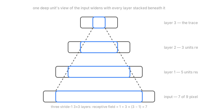
The diagram above traces this by hand, on a simplified one-dimensional strip of nine input units, through three stacked 3×3 convolutions (stride 1, no padding). Start at the single traced unit in the third layer. It was computed from three units in the layer below — that's just what a 3×3 kernel does, it reads three positions. Each of those three units was itself computed from three units in the layer below them, and because the three windows overlap, their union covers five units, not nine. Repeat once more and the union across the input reaches seven of the nine original positions.

Three layers, and the reachable footprint grew 3 → 5 → 7: a jump of two units per layer, matching the kernel's own width minus one. That's not a coincidence — it's the rule.

The formula, and why it's additive

For $L$ stacked layers, each with kernel size $k$ and stride 1, the receptive field is:

Plug in the diagram's numbers — three layers of kernel size 3 — and $\text{RF} = 1 + 3 \times 2 = 7$, exactly what the traced diagram shows. The growth is additive with depth for stride-1 layers: each extra layer adds a fixed $(k-1)$ to the field, not multiplies it. That's a meaningfully slow rate. It's the reason early CNNs needed real depth — a dozen or more layers — before a unit's field covered anything close to a whole typical input image.

Two things that grow the field faster than plain stacking

Pooling and strided convolutions grow the field multiplicatively, not additively. Downsampling shrinks the map, so every kernel applied afterward is reading from a coarser grid where each cell already represents a larger patch of the original input. A pooling layer with stride 2 roughly doubles the effective receptive field of everything that comes after it, which is a big part of why real architectures interleave downsampling with convolutions rather than stacking dozens of stride-1 layers back to back.

Dilation grows the field without adding parameters or depth at all. A dilated 3×3 kernel with dilation rate $r$ spreads its three taps across a span of $1 + 2r$ positions instead of 3, so its effective kernel size for the receptive-field formula becomes $k_{\text{eff}} = k + (k-1)(r-1)$. Swap that into the same additive formula and one dilated layer can cover as much ground as several ordinary ones — the trade being that the kernel now skips positions in between rather than reading every one of them.

Effective versus theoretical

The formula above gives the theoretical receptive field — every input position a unit is mathematically connected to. In practice, not every position inside that field influences the output equally: positions near the center of the field, reached through many overlapping paths, tend to matter far more than positions right at the edge, reached through only one. The effective receptive field is smaller than the theoretical one and, in well-trained networks, tends to look roughly Gaussian — concentrated in the middle, fading toward the edges. The formula tells you the field's outer boundary; it doesn't tell you how much each pixel inside that boundary actually counts.

Show Me the Code

Computing the theoretical receptive field for a stack of layers, mixing plain convolutions with a downsampling stage.

1def receptive_field(layers: list[tuple[int, int]]) -> int:2    """Each layer is (kernel_size, stride). Returns the theoretical RF at the top."""3    rf, jump = 1, 1  # jump tracks how many input pixels one output step represents4    for kernel_size, stride in layers:5        rf += (kernel_size - 1) * jump6        jump *= stride7    return rf8
9
10three_stride1 = [(3, 1), (3, 1), (3, 1)]11print(receptive_field(three_stride1))  # -> 7  (matches the diagram: 1 + 3*(3-1))12
13with_downsampling = [(3, 1), (2, 2), (3, 1), (3, 1)]  # a stride-2 pool after the first layer14print(receptive_field(with_downsampling))  # -> 12

Trace with_downsampling step by step and the multiplicative effect is visible directly: the first 3×3 layer takes the field from 1 to 3. The stride-2 pool adds only 1 more (its own kernel size minus one, times the current jump of 1) but doubles the jump to 2 — and from there, each remaining 3×3 layer adds $(3-1) \times 2 = 4$ instead of 2. The last two layers alone contribute 8 of the total 12, exactly because the pool doubled what each subsequent layer is worth.

Watch Out For

The Quick Version

• A single kernel sees only its own small patch. The receptive field is how much of the original input a unit depends on once you trace back through every layer beneath it.
• For stacked stride-1 layers, the field grows additively: $\text{RF} = 1 + L(k-1)$.
• Pooling and strided convolutions grow the field multiplicatively, because every later layer reads from an already-shrunk map.
• Dilation grows the field without adding depth or parameters, by spreading the kernel's taps apart.
• The effective receptive field — what actually drives the output — is smaller than the theoretical one and concentrates toward the center.

What to Read Next

• Convolution Operation is the single-layer mechanism this page stacks.
• Pooling Layers is the multiplicative growth lever this page relies on.
• Convolutional Neural Networks is the full architecture where receptive field size becomes a real design decision.
• CNN Architecture Lineage shows how successive architectures managed receptive field growth differently.
• Residual Connections is what made it practical to add enough layers to grow the field this way without the network becoming untrainable.