Core ML

Quantile Regression

Fit a line that a chosen fraction of outcomes fall below, instead of the average outcome — predicting a spread instead of one collapsed number.

Three fitted lines split a scattered, fanning-out cloud of points differently — the median line sits centered, the 10th-percentile line runs beneath most points, and the 90th-percentile line runs above most of them

Why Does This Exist?

A delivery company wants to promise a delivery window, not just an average delivery time. Linear regression fits the mean delivery time given distance — useful for planning fleet capacity, useless for a customer who wants to know "by when will this arrive, with reasonable confidence." Worse, delivery times don't spread evenly: short trips are consistently quick, while long trips vary enormously depending on traffic, weather, and route — the spread itself grows with distance, a pattern called heteroscedasticity. One mean prediction, with one implied margin of error, doesn't capture that a long trip's uncertainty is genuinely larger than a short trip's.

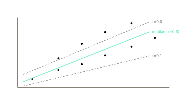
Quantile regression fits a different line for each question actually worth asking: not "what's the average delivery time," but "what delivery time will 90% of trips beat" — a line for the median, a line for a conservative 90th-percentile estimate, each fit directly rather than derived from a single mean-and-variance assumption.

Think of It Like This

Three referees with different standards for 'good enough'

Imagine three referees judging the same set of dives, each with a completely different tolerance. One referee passes exactly half the dives — this is the "median" referee, splitting the field evenly. A second referee is lenient, passing 90% of dives — only the worst 10% fail their bar. A third is strict, passing only 10% — a very high bar to clear.

Each referee, given the same dives, draws their own line for "how good is good enough," and the three lines don't move together in any simple way — the gap between the lenient and strict referee's bars can widen or narrow across different divers depending on how consistent each diver's performance actually is. Quantile regression fits exactly this: several different "bars," each answering a different question about the same underlying data.

How It Actually Works

The pinball loss: an asymmetric penalty

Ordinary linear regression minimizes squared error, which penalizes overshooting and undershooting the true value equally — appropriate for estimating a mean. Quantile regression at quantile $\tau$ (for example $\tau = 0.9$ for the 90th percentile) instead minimizes the pinball loss:

L_\tau(y, \hat{y}) = \begin{cases} \tau (y - \hat{y}) & \text{if } y \geq \hat{y} \\ (\tau - 1)(y - \hat{y}) & \text{if } y < \hat{y} \end{cases}

For $\tau = 0.9$ , underestimating the true value ( $y \geq \hat{y}$ ) costs 0.9 times the gap, while overestimating costs only 0.1 times the gap — a strong asymmetric penalty for being too low, which pushes the fitted line up until exactly 90% of points sit at or below it. Setting $\tau = 0.5$ recovers a symmetric penalty and produces the median line, matching the intuition that a median split treats over- and under-estimates identically.

Why the fitted line ends up where it does

At the loss's optimum, the fraction of training points falling below the fitted line converges to exactly $\tau$ — this is the entire mechanism, and it's what makes $\tau = 0.9$ produce a genuine 90th-percentile line rather than an approximation of one. Because each quantile is fit independently, with its own asymmetric loss, quantile regression captures heteroscedasticity directly: if the spread between the 10th- and 90th-percentile lines widens as the input grows, that widening is read straight off the data, with no explicit variance model required anywhere.

What this buys over a mean-and-variance approach

A traditional approach models the mean and assumes a fixed-shape spread around it — often a symmetric normal distribution, which fails badly when the real spread is skewed or heteroscedastic, exactly the delivery-time case above. Quantile regression makes no such assumption: each quantile is fit on its own terms, so a genuinely skewed or unevenly-spread outcome distribution is captured without needing to specify its shape in advance.

Show Me the Code

Fitting the median, 10th-percentile, and 90th-percentile lines on data whose spread grows with the input, and confirming the 90th-percentile line's coverage.

1import numpy as np2
3rng = np.random.default_rng(1)4n = 20005x = rng.uniform(0, 10, n)6y = 2 * x + rng.normal(0, 1, n) * (0.5 + 0.5 * x)  # spread grows with x7
8
9def fit_quantile(x: np.ndarray, y: np.ndarray, tau: float, steps: int = 2000, lr: float = 0.01) -> tuple[float, float]:10    w, b = 0.0, 0.011    for _ in range(steps):12        residual = y - (w * x + b)13        grad_sign = np.where(residual >= 0, -tau, -(tau - 1))14        w -= lr * np.mean(grad_sign * x)15        b -= lr * np.mean(grad_sign)16    return w, b17
18
19for tau in (0.1, 0.5, 0.9):20    w, b = fit_quantile(x, y, tau)21    print(f"tau={tau}: y = {w:.3f}*x + {b:.3f}")22
23w90, b90 = fit_quantile(x, y, 0.9)24coverage = np.mean(y <= w90 * x + b90)25print(f"fraction of points at or below the tau=0.9 line: {coverage:.3f}")26# -> tau=0.1: y = 1.289*x + -0.27927# -> tau=0.5: y = 1.972*x + 0.11728# -> tau=0.9: y = 2.606*x + 0.65229# -> fraction of points at or below the tau=0.9 line: 0.894

The median line's slope of 1.972 sits close to the data's true slope of 2. The 10th- and 90th-percentile lines diverge from it in opposite directions, and their gap — visible directly in the different slopes — is exactly what captures the growing spread. The measured coverage of 89.4% confirms the mechanism directly: fitting at $\tau = 0.9$ really does produce a line roughly 90% of points fall below.

Watch Out For

Fitting quantiles independently and getting crossing lines

Because each quantile is optimized separately, nothing in the basic method guarantees the 90th-percentile line stays above the median line everywhere — with limited data or an unstable fit, the lines can cross, producing the nonsensical claim that the 90th percentile is sometimes lower than the median. Specialized fitting procedures that jointly constrain multiple quantiles exist specifically to prevent this; check for crossing whenever fitting several quantiles independently on real data.

Treating a quantile prediction as a probability statement about one specific case

A 90th-percentile prediction says that, across many similar cases with similar inputs, roughly 90% of outcomes fall at or below that line — it is not a guarantee about any single future case, which could still land above it. Communicate quantile predictions as intervals with a stated confidence level, not as hard upper bounds.

The Quick Version

Quantile regression fits a separate line for each quantile of interest, using the asymmetric pinball loss instead of squared error.
At $\tau = 0.5$ it recovers median regression; at other values of $\tau$ it directly estimates a chosen percentile of the outcome distribution.
It captures heteroscedasticity — spread that changes with the input — directly from the data, without assuming a fixed distribution shape.
Independently-fit quantile lines can cross with limited data, since nothing in the basic method enforces that a higher quantile stays above a lower one.