Core ML

Statistical Learning Theory

A generalization bound caps how far true error can exceed training error — and the honest catch is that cap is usually far too loose to use as a real number.

A generalization bound curve falls sharply as sample size grows, showing why more data shrinks the gap between training and true performance, even though the bound's own numeric value is far too loose to use directly

Why Does This Exist?

Overfitting and underfitting teaches how to spot the symptom: a widening gap between training and validation performance. What it doesn't answer is a harder question underneath: is there a way to guarantee, before ever touching a validation set, how far a model's training performance can possibly be from its true performance on data it hasn't seen? Statistical learning theory exists to answer that question — not with intuition, but with a mathematical bound that holds regardless of which specific dataset you happened to get.

The honest headline result deserves saying upfront: the bounds this field produces are almost always far too loose to plug in a number and act on directly. What survives, and what actually earns this page a place in the curriculum, is the shape of the argument — why more data reliably helps, why model capacity has a real cost, and why skipping a held-out test set is never safe no matter how good training performance looks.

Think of It Like This

A worst-case weather forecast versus a useful one

A forecaster who guarantees "there is a mathematically provable chance of anywhere from 0% to 100% rain tomorrow" has said something true and completely useless as a number. But buried in that same reasoning is something genuinely useful: as more weather stations report in, that provable range shrinks, and it shrinks faster the simpler the weather pattern being tracked. The exact bound is worthless as a forecast. The relationship — more data narrows the guarantee, and simpler patterns narrow it faster — is the real content.

Statistical learning theory's generalization bounds work the same way: the specific number they output is rarely tight enough to trust directly, but the relationships they prove — more samples help, more model capacity costs you, in a specific tradeoff — are exactly right and exactly why they're studied.

How It Actually Works

PAC learning: probably, approximately correct

PAC learning (Probably Approximately Correct) frames the question precisely: given $n$ training examples, what's the probability that a model's true error exceeds its training error by more than some margin $\epsilon$ ? "Probably" acknowledges that any finite sample could be unlucky — there's always some small probability $\delta$ the bound fails entirely. "Approximately" acknowledges the bound targets being close to correct, not exactly correct. This framing is what makes a provable, distribution-free guarantee possible at all: it never claims certainty, only a bounded probability of being meaningfully wrong.

VC dimension: measuring how much a model class can memorize

The VC dimension (Vapnik–Chervonenkis dimension) of a model class measures its raw capacity to fit arbitrary patterns — the largest number of points that class can label in every possible way, regardless of arrangement. A class with VC dimension 3 can shatter — correctly classify under every labeling — any 3 points in general position, but not every arrangement of 4. Higher VC dimension means more flexibility to fit training data, exactly the property that makes overfitting possible: a class flexible enough to fit anything is flexible enough to fit noise.

The generalization bound, and why it's loose

A representative PAC-style bound looks roughly like:

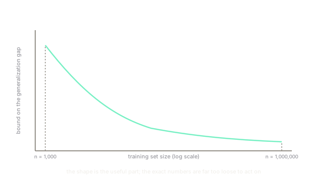
\text{true error} \leq \text{training error} + \sqrt{\frac{d \left(\log\frac{2n}{d} + 1\right) + \log\frac{4}{\delta}}{n}}

$d$ is the VC dimension, $n$ is the sample count, and $\delta$ is the small failure probability. What matters is the shape: the gap term shrinks as $n$ grows, and grows as $d$ grows — precisely the tradeoff bias–variance describes from a different angle. The catch is that this bound assumes nothing about the data's real distribution, which is exactly what makes it universally valid and exactly what makes it numerically enormous — a bound that has to hold for every conceivable data distribution simultaneously cannot be tight for any specific one.

What survives contact with practice

Nobody computes this bound and reports "true error is at most X" — the number typically says something like "at most 30 percentage points worse," true and worthless. What survives is the reasoning skeleton: more data provably tightens the gap between measured and true performance, more model capacity provably costs you in that same gap, and no amount of training-set performance is a substitute for measuring on unseen data. That last point isn't experience talking; it's the direct consequence of what the bound claims.

Show Me the Code

The bound's shape, computed at a fixed model capacity across a range of sample sizes.

1import numpy as np2
3
4def pac_bound(vc_dim: int, n_samples: int, delta: float = 0.05) -> float:5    """A representative PAC-style generalization-gap bound."""6    term = (vc_dim * np.log(2 * n_samples / vc_dim) + np.log(4 / delta)) / n_samples7    return float(np.sqrt(term))8
9
10for n in (1_000, 10_000, 100_000, 1_000_000):11    bound = pac_bound(vc_dim=10, n_samples=n)12    print(f"n={n:>9,}: bound on the gap = {bound:.4f}  (up to {bound * 100:.1f} percentage points)")13# -> n=    1,000: bound on the gap = 0.2395  (up to 24.0 percentage points)14# -> n=   10,000: bound on the gap = 0.0897  (up to 9.0 percentage points)15# -> n=  100,000: bound on the gap = 0.0322  (up to 3.2 percentage points)16# -> n=1,000,000: bound on the gap = 0.0112  (up to 1.1 percentage points)

Even at a million samples with a modest VC dimension of 10, the bound still allows for a gap of over a full percentage point — for many real applications, still too loose to act on as an exact number. What it demonstrates cleanly is the rate: a ten-fold increase in data doesn't shrink the bound ten-fold, it shrinks it by roughly the square root of ten, which is the concrete shape behind "more data helps, with diminishing returns."

Watch Out For

Quoting a generalization bound as an actual accuracy guarantee

A PAC bound of "at most 24 percentage points worse than training error" is true and is not a useful accuracy promise to make to a stakeholder — the looseness is inherent to the bound being valid for every possible data distribution, not a sign that the math was done wrong. Use held-out validation and test sets for any real accuracy claim; use the theory for the reasoning about why those held-out sets are non-negotiable in the first place.

Assuming VC dimension alone predicts real-world overfitting risk

VC dimension measures worst-case capacity assuming an adversarial data arrangement, and real datasets are rarely adversarial. Deep neural networks routinely have VC dimensions far higher than their parameter count would suggest is safe, and yet generalize well in practice — a gap between the classical theory and observed behavior that's still an active area of research. Treat VC dimension as one input to intuition about capacity, not a precise real-world overfitting predictor.

The Quick Version

PAC learning frames generalization as a probabilistic guarantee: with high probability, true error won't exceed training error by more than a bounded margin.
VC dimension measures a model class's raw capacity to fit arbitrary labelings, and higher VC dimension both enables more overfitting and worsens the generalization bound.
The bound's numeric value is almost always too loose to use directly, because it must hold for every possible data distribution at once.
What survives practically: more data narrows the gap, more capacity widens it, and a held-out test set is never optional — all consequences of the bound's actual shape, not empirical folklore.