Core ML

Stochastic Gradient Descent

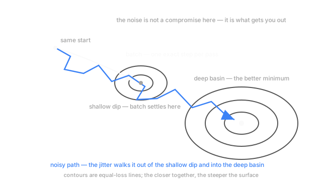
One row per step instead of all of them looks like a shortcut. The wobble it adds is doing real work: it walks the model out of shallow dips and saddles.

On the same loss surface from the same start, an exact-gradient path slides into the nearest shallow dip and stops, while a noisy one-row-at-a-time path wanders out of that dip and reaches the deeper basin

Why Does This Exist?

Estimating something from one example instead of sixty thousand sounds like the worse plan. For training a model it isn't, and speed is only half the reason.

Our example down the page: 60,000 handwritten digit images and a classifier that has to name each one. The file they arrive in is sorted by label, all the zeros then all the ones, which will matter later. Two words training logs conflate constantly. A step is one parameter update. An epoch is one full pass over all 60,000 images. Batch gradient descent gets one step per epoch. Stochastic gradient descent gets 60,000, each from a single image.

A rough gradient many times over an exact gradient once — that's what "stochastic" buys. The interesting part is that the roughness is useful on its own terms.

Think of It Like This

Shaking a tray of marbles

A baking tray pressed with dimples of different depths, marbles rolled across it. Hold the tray still and every marble stops in the first dimple it meets, most of them shallow. Shake it gently: the marbles in shallow dimples hop out and keep travelling, and the ones in deep dimples stay, because the shake can't lift them that far.

The shake isn't sloppy tray-holding. It's the mechanism — the only thing separating a marble in a good dimple from one in a poor dimple it happened to reach first. Shake too hard and nothing settles anywhere.

That shake is the gradient noise from looking at one image at a time.

How It Actually Works

The update looks the same as before:

\theta_{t+1} = \theta_t - \eta \nabla_\theta L_i(\theta_t)

with one change. $L_i$ is the loss on a single image $i$ , not the average over all 60,000, and $\nabla_\theta L_i$ is its gradient with respect to the parameters $\theta$ . Draw $i$ uniformly at random and that gradient equals the full-data gradient in expectation. Every step points roughly the right way and no step points exactly the right way.

The noise is doing work

An exact gradient at a saddle point is a dead end. The gradient is near zero, so the step is near zero, and you sit there. Same for a shallow basin: the walls point inward from every side and batch descent has no way out. Per-example gradients disagree with each other, so a one-image estimate at that same point is not near zero, and it pushes you somewhere else. Then again, differently.

The second effect is subtler and probably matters more. The noise scale behaves like a regulariser nobody wrote down. A high-noise run can't stay in a narrow basin — the jitter keeps knocking it out — so it ends up in a wide flat one. Flat minima generalise better, because a small shift between your training data and next month's data moves the loss less when the floor around you is level. That bias toward flatness falls out of the sampling, not the objective.

Shuffling isn't optional

Now the sorted file matters. Ten thousand consecutive steps drawn from a block of zeros all say the same thing: predict zero, harder. That's not a random walk. It's a systematic drift, and the parameters ride it a long way before the ones show up and drag them back.

The tell is a loss curve with a ripple whose period matches the epoch boundary. Shuffle before every epoch and the drift becomes noise again, which is the whole thing you wanted.

Batch size, noise, and the rate

Gradient noise falls with the square root of the batch size. Quadruple the batch and you halve the noise. Which means a very large batch is close to batch descent: accurate, and stripped of the regularising jitter that was quietly helping.

The standard patch is the linear scaling rule: scale the learning rate with the batch size, so doubling the batch doubles the rate. That holds roughly the same movement per epoch and the same noise relative to step size. It works over a wide range and then stops — past a critical batch size, extra rows per step buy almost nothing and the rate needed to compensate destabilises the run. Where that point sits is model-specific, and you find it by measuring.

Show Me the Code

The square-root law, measured. Fix the parameters, then see how much the gradient estimate scatters across draws.

1import numpy as np2
3rng = np.random.default_rng(1)4n: int = 60_0005x: np.ndarray = rng.normal(0.0, 1.0, n)6y: np.ndarray = 3.0 * x + rng.normal(0.0, 1.0, n)   # one weight, true value 3.07
8
9def grad_spread(batch: int, w: float = 0.0, draws: int = 6000) -> float:10    g = np.empty(draws)                             # the noise one step actually sees at fixed w11    for d in range(draws):12        i = rng.integers(0, n, batch)13        g[d] = 2.0 * float(((w * x[i] - y[i]) * x[i]).mean())14    return float(g.std())15
16
17spread: dict[int, float] = {b: grad_spread(b) for b in (1, 4, 16, 64)}18for b, s in spread.items():19    print(f"batch {b:>3}  gradient std {s:5.2f}   share of the batch-1 noise {s / spread[1]:.2f}")20    # -> batch   1  gradient std  8.83   share of the batch-1 noise 1.0021    # -> batch   4  gradient std  4.31   share of the batch-1 noise 0.4922    # -> batch  16  gradient std  2.18   share of the batch-1 noise 0.2523    # -> batch  64  gradient std  1.09   share of the batch-1 noise 0.12

Sixty-four times the work for eight times less noise. That ratio is why nobody runs batch size 1 — or 60,000.

Watch Out For

Order that comes from the file, not from a shuffle

Symptom: the loss curve has a periodic ripple lining up with the epoch boundary, and two runs with different seeds behave differently in ways that don't look like seed noise. Streaming pipelines hide this well, because data that arrives grouped by day, by source, or by customer never passes through a shuffle at all.

Every step in a grouped stretch pulls the same direction, so the model drifts toward whatever that group wants and then gets dragged back. Shuffle each epoch for a dataset you hold; for a stream, buffer a few thousand records and sample from the buffer. The fix costs almost nothing, and the failure is invisible until you compare against a shuffled baseline.

Raising the batch size for throughput and leaving the rate alone

Symptom: you move from 64 to 512 to fill the GPU, training gets faster per epoch, training loss looks fine, and validation accuracy comes out slightly worse. Nothing errored, so nothing gets investigated.

Eight times the batch cut the gradient noise to roughly a third, and you deleted regularisation you didn't know you had. Scale the rate up with the batch, warm it up over the first few hundred steps so the larger rate doesn't blow up early, and re-check validation rather than training loss. If the gap survives at the scaled rate, you're past the critical batch size and the throughput win isn't free.

The Quick Version

Same update as gradient descent, computed from one example or a small batch instead of the whole dataset.
That gradient equals the true one in expectation, so every step is right on average and wrong individually.
The noise is a feature: it escapes saddle points and shallow basins where an exact zero gradient sits forever.
It also biases the search toward flat minima, which generalise better. Free regularisation, unwritten.
Shuffle every epoch. Data grouped by class or source turns noise into drift, and the tell is a ripple at the epoch boundary.
Noise falls with the square root of batch size, so scale the rate with the batch — until the critical batch size, where that stops holding.