Data Concepts

Data Imputation

Every filled gap is a value you made up. The model can't tell it from a measurement, and your variance and correlations both shift the moment you do it.

Mean imputation does not fill the gaps neutrally: it stacks every filled row into one bar at the mean, shrinking the column's variance and pulling its correlation with everything else toward zero

Why Does This Exist?

SimpleImputer(strategy="mean") writes a number into a cell where no measurement exists. The model then reads that cell exactly the way it reads a real one. There is no flag, no weight, no note in the margin. A fabricated 4.0 and a measured 4.0 are the same float.

That reframes the usual question. "Which imputation method is best" has no answer, because none of them recover the value — they can't, the value is gone. The question that does have an answer: what damage does this method do to the column, and does the model get told a value was fabricated? The damage is measurable in advance. The telling costs one extra column.

Everything below assumes you know why the cells are blank. If you don't, read missing data first, because the mechanism decides which of these methods is defensible and which is quietly indefensible.

Think of It Like This

A restorer filling a hole in a painting

A canvas comes into the studio with a patch of paint flaked away. The restorer mixes a colour from what surrounds the hole and fills it in. Stand back and you cannot see the join — that's the craft.

Now a researcher arrives to study the painter's palette. They sample pigment across the canvas and report an average, and their average is partly the restorer's guess. They can't tell which readings are original, so the guess enters the finding at full weight — and the more the restorer filled, the more the finding is about the studio rather than the painter.

Conservation solved this long ago. Reversible materials, and a written record of every retouched region, so a later analyst can exclude them. The filling still happens. It just stops pretending to be evidence.

Your imputer is the restorer. Your model is the researcher. The written record is one boolean column, and it's the cheapest thing on this page.

How It Actually Works

A ladder, in rough order of cost and assumption. Climb only as far as the problem forces you.

Leave it missing. LightGBM, XGBoost and scikit-learn's HistGradientBoosting all take NaN directly. At each split they learn which branch the missing rows should take, so "absent" becomes a value the tree can act on. Frequently the best answer on tabular data, and skipped almost universally because a pipeline with an imputer in it looks more finished. Try it first and measure.

A constant, plus an indicator. Fill with a value outside the real range and add a boolean column marking where you filled. Honest, cheap, fine for trees. Linear models read the constant as a magnitude, so keep it in a sane range or use them elsewhere.

Mean or median. One number for the whole column. Use the median whenever the column is skewed — latency, income, spend, session length, counts — because the mean of a long-tailed column sits above most of the data, and descriptive statistics shows how far above. Mean is defensible on symmetric columns and nowhere else.

Mode, or a category called "Missing". For categorical columns the explicit category usually wins. Mode imputation hands the blanks to whichever level was already most common, inflating it and erasing the fact that anything was absent. A "Missing" level keeps that, and categorical encoding carries it downstream like any other.

Group-wise statistics. Median income within (region, job_title) rather than overall. Cheap, often much better, and the practical way to use a MAR mechanism: you're conditioning on the columns the gaps depend on. Watch the small groups — a median from three rows is noise with a decimal point.

KNN imputation. Average the value from the $k$ nearest complete rows, measured across the other columns. Needs scaled inputs, since the search uses distance, and it costs $O(n^2)$ comparisons, which rules it out past tens of thousands of rows.

Iterative, also called MICE. Model each gapped column as a regression on all the others, cycle through them, repeat until the values settle. The strongest of these on MAR data and the slowest by a wide margin.

Forward-fill, for time series only. Carry the last observed value forward. Correct for a reading you'd genuinely have had, and a leak the moment it crosses a train/test boundary: fill across a chronological split and a test-period gap inherits a training-period value, which is information travelling backwards in time. Fill within each segment, never through the cut.

Every one of these is fitted

The mean, the median, the group medians, the neighbour set, the MICE regressions — all learned from rows. So the rule from feature scaling carries over unchanged: fit on training rows, apply everywhere, refit inside every cross-validation fold. Put the imputer in a Pipeline and hand that to the cross-validator, so it stops being something you remember.

What mean imputation does to the column

Not a side effect. Arithmetic.

Variance is the total squared distance from the mean, divided by the number of rows. A value placed exactly at the mean contributes zero to that total. So the numerator holds still while the denominator grows:

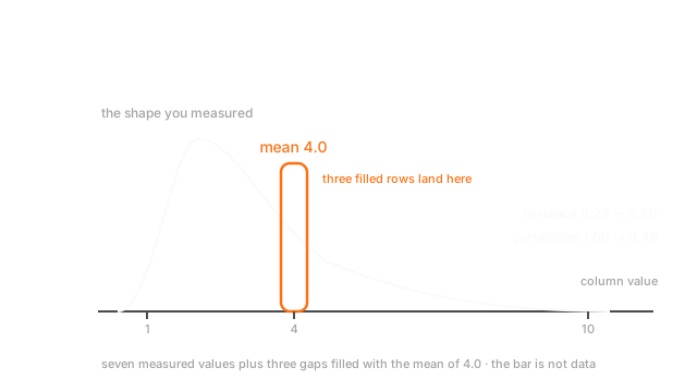
\frac{58}{7} = 8.29 \quad \longrightarrow \quad \frac{58}{10} = 5.80

Here 58 is the total squared distance from the mean across the seven measured values, 7 becomes 10 as three gaps get filled, and the variance falls 30% without a single measurement changing. Every downstream interval, significance test and variance-based selection score is now wrong in a known direction.

Correlation goes the same way, harder. It needs the two columns to move together, and a spike of identical values can't move with anything. Three rows sharing one $x$ against three different $y$ values add nothing to the numerator and plenty to the denominator, so the coefficient falls toward zero. You're weakening the exact relationship you built the column to expose.

Worked example

One column $x$ with seven measured values — 1, 2, 2, 3, 4, 6, 10 — and three gaps. A second column $y$ running 2, 4, 4, 6, 8, 12, 20 on those seven rows, so $y = 2x$ exactly and the correlation among measured pairs is 1.00. The three gapped rows carry $y$ of 24, 26 and 30.

The measured values sum to 28, so the mean is $28/7 = 4.0$ and the median is 3.0. Fill with the mean and $x$ becomes 1, 2, 2, 3, 4, 6, 10, 4, 4, 4. Variance drops from 8.29 to 5.80, as above. Correlation with $y$ drops from 1.00 to 0.49.

Fill with the median instead and it falls further, to 0.32. That's not median imputation being worse in general — it's this mechanism biting. The gapped rows are the high- $y$ rows, so a lower fill sits further from where those rows belong. Which fill hurts least depends on why the gaps are there.

Show Me the Code

1import numpy as np2
3x = np.array([1, 2, 2, 3, 4, 6, 10, np.nan, np.nan, np.nan])4y = np.array([2, 4, 4, 6, 8, 12, 20, 24, 26, 30])5seen = ~np.isnan(x)6
7
8def fill(col: np.ndarray, value: float) -> np.ndarray:9    """A fabricated value the model cannot tell apart from a measured one."""10    return np.where(np.isnan(col), value, col)11
12
13mean_fill = fill(x, float(np.nanmean(x)))      # a constant 4.0 in three rows14median_fill = fill(x, float(np.nanmedian(x)))  # a constant 3.0 in three rows15
16print(round(x[seen].var(), 3), mean_fill.var())        # -> 8.286 5.817print(round(np.corrcoef(x[seen], y[seen])[0, 1], 2))   # -> 1.018print(round(np.corrcoef(mean_fill, y)[0, 1], 3))       # -> 0.48619print(round(np.corrcoef(median_fill, y)[0, 1], 3))     # -> 0.316

A perfect linear relationship became a mediocre one, and nothing was measured wrong. Three rows out of ten did that.

Watch Out For

Fitting the imputer on the whole frame

SimpleImputer().fit_transform(X) and then train_test_split. It reads better than the correct order, which is why it's the most common leak in tabular work.

The median you just computed contains your test rows, and it gets written into training cells. Validation improves. Production doesn't.

Mechanically this is the same leak as fitting a scaler too early, and worse in effect. A scaler shifts and stretches a column every row shares; an imputer writes the leaked statistic into individual cells as their value. At 30% missing, nearly a third of that training column is literally a test-set summary. Group-wise and iterative imputers carry more leaked structure per cell, so they're sharper still.

Fix it structurally: every fitted step inside a Pipeline, the pipeline passed to the cross-validator, refit per fold. See cross-validation schemes for what "per fold" has to mean when rows are grouped or ordered in time.

Imputing the target, or imputing after you've derived a feature

Two mistakes with the same shape: fabricated numbers ending up somewhere they can't be detected.

Filling gaps in the target is not modelling. Whatever you fill with, you're training the model to reproduce your imputer, and your score partly measures how well it learned that. Unlabelled rows get dropped from supervised training, or moved into a semi-supervised setup where their status is explicit. There's no third option.

Order is the subtler one. Compute spend_per_visit = spend / visits, impute the gaps in spend afterwards, and the ratio is already NaN on those rows — or worse it isn't, because someone imputed spend in a copy of the frame and the derived column inherited the guess. The fabricated value has propagated into a column with no indicator on it, and it looks like an ordinary ratio.

So fix the order and write it down: indicators first, nulls resolved second, derived columns last. Then audit the derived columns, because a feature that inherited fabricated values shows nothing unusual in a histogram.

The Quick Version

Imputation invents values. The model can't distinguish them from measurements, so pick by the damage done, not by which method sounds strongest.
Try leaving the gaps in. LightGBM, XGBoost and HistGradientBoosting take NaN and learn a direction for it, and that gets skipped far too often.
Median for skewed numeric columns, mean only for roughly symmetric ones. An explicit "Missing" category usually beats the mode.
Group-wise medians are the cheap way to use a MAR mechanism. KNN needs scaled columns and stops scaling past tens of thousands of rows. MICE is strongest and slowest.
Forward-fill is for time series, within a segment. Across a train/test cut it leaks.
Add a missingness indicator whatever you choose. One column, and the fabrication becomes visible to the model.
Mean imputation cuts variance by construction: the numerator holds at 58 while the row count goes 7 to 10, so 8.29 becomes 5.80.
It flattens correlation too. A perfect 1.00 fell to 0.49 from three filled rows out of ten.
Every imputer is fitted. Fit on training rows, refit inside every fold, and never on the target.