Data Concepts

Dimensionality Reduction

One question sorts every method here: does it hand you a transform you can apply to a new row? PCA does. t-SNE never will, which is why it stays a plot.

PCA finds the cloud's long axis first and an orthogonal direction second, so projecting onto that first component keeps almost all the spread and costs one column

Why Does This Exist?

TF-IDF twenty thousand support tickets and you get a matrix 38,000 columns wide. Nothing is wrong with it. It also can't be plotted and makes anything distance-based unreliable, because at that width every pair of points sits at roughly the same distance apart (sparse data and high dimensionality).

Two reasons to want fewer columns. Preprocessing: fewer inputs to a model that runs next month, on rows nobody has collected yet. Looking: two axes on a screen, so you can see whether your classes separate at all.

One question sorts them: does the method hand you a transform you can save and apply to a single new row? PCA does, LDA and TruncatedSVD do, t-SNE and UMAP don't. Pretending otherwise is the most common misuse here.

Think of It Like This

A shadow on the wall and a seating plan

Hold a wire chair in front of a lamp. The shadow lost the depth, but the rule that made it is fixed: lamp there, wall here. Bring a second chair and its shadow appears under the same rule. That rule is a transform, the part you can ship.

Different job. Forty guests, and you shuffle the seating until friends sit close and strangers sit apart. The cliques are visible at a glance. Then guest forty-one turns up, and there's no rule to apply — the plan came out of the relationships among those forty. The gap between two tables measures nothing either.

Shadows are PCA. Seating plans are t-SNE.

How It Actually Works

PCA, and what maximum variance buys

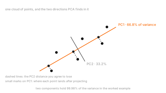
Centre every column on its mean, then find the direction along which the projected points spread out most. That's the first principal component; the second is the direction of most remaining spread at a right angle to it. Those directions are the eigenvectors of the covariance matrix sorted by eigenvalue, equivalently the right singular vectors of the centred matrix (SVD). Each eigenvalue over their sum is that component's variance share, so you keep components until the total hits your target.

Neither input requirement is optional. Centre: variance is measured about the mean, and PCA has no other origin. Scale: variance carries units, so a column in centimetres outvotes the same column in metres 10,000 to one (feature scaling).

The others that hand you a transform

TruncatedSVD takes those same singular vectors without centring, which is why it runs straight on a sparse matrix — centring would fill in every zero. It's what you use on TF-IDF, where it goes by latent semantic analysis.

LDA maximises between-class over within-class scatter instead of variance, so it's capped at one fewer component than you have classes. It reads the labels, so fitting it outside the fold leaks like a target encoder (cross-validation schemes).

Random projection multiplies by a random matrix and stops. Johnson–Lindenstrauss says that's enough: 10,000 points with distances held within ±50% needs 442 dimensions, and ten times the points costs 110 more. Nothing is fitted, so nothing leaks. The learned non-linear version is an autoencoder bottleneck, at the price of a training run — that's the door into latent spaces and manifold learning.

The two that don't

t-SNE and UMAP build a neighbour graph, then arrange points in two dimensions so neighbours stay neighbours. Local structure survives. Global structure doesn't, and three things on those plots carry no information. Cluster size: a tight blob and a sprawling one can hold the same spread. Distance between clusters: opposite corners aren't more different than touching blobs. Apparent gaps: that's where the layout ran out of pressure.

One knob changes the answer: perplexity in t-SNE, n_neighbors in UMAP. Turn it up and blobs merge, turn it down and one shatters into five. Diagnosis tools, and never a pipeline stage.

Worked example

Three columns on 300 people: height in centimetres, the same height in inches with a tenth of an inch of noise, and resting heart rate.

Standardise, run PCA, and the variance shares come out 66.81%, 33.17% and 0.01%. Two components hold 99.98%, because a third independent column was never there. Loadings on the first are 0.705, 0.705, 0.069: equal weight on the height pair, since $1/\sqrt{2} = 0.707$ , and heart rate barely registering.

Skip the standardising and those loadings become 0.929, 0.366, 0.056. Divide the first by the second: 2.54, the centimetres in an inch. Nothing about the data changed.

Show Me the Code

1import numpy as np2
3rng = np.random.default_rng(0)4height_cm = rng.normal(170.0, 9.0, 300)5height_in = height_cm / 2.54 + rng.normal(0.0, 0.1, 300)  # same fact, different ruler6X = np.column_stack([height_cm, height_in, rng.normal(68.0, 7.0, 300)])7
8
9def pca(data: np.ndarray) -> tuple[np.ndarray, np.ndarray]:10    """Centre, take the singular values, square them. Loading signs are arbitrary."""11    _, s, vt = np.linalg.svd(data - data.mean(axis=0), full_matrices=False)12    return 100 * s**2 / (s**2).sum(), np.abs(vt[0])13
14share, pc1 = pca(X / X.std(axis=0))         # standardised, which is how to run it15print([round(float(v), 2) for v in share])  # -> [66.81, 33.17, 0.01]16print(np.round(pc1, 3))                     # -> [0.705 0.705 0.069]17print(np.round(pca(X)[1], 3))               # -> [0.929 0.366 0.056]

One expression separates those results: X / X.std(axis=0). Drop it and PC1 describes your unit rather than your data.

Watch Out For

Reading structure off a t-SNE or UMAP plot

Six well-separated blobs come back, two far apart on the right, and "segments 3 and 5 are the most distinct" goes into the summary. That claim was never in the data: positions came from a stochastic layout that only tried to keep near neighbours near, and dropping perplexity from 30 to 5 turns six blobs into fifteen.

The worse version happens next. You keep the two output columns and hand them to a classifier. There's no transform for a new row, so it can't be served, and the layout saw every row you own, so the score was inflated before the classifier started. Want two columns feeding a model? PCA or TruncatedSVD, inside the fold.

PCA on unscaled columns, fitted before the split

Both bugs come out of PCA().fit(X) on the raw frame.

The scaling half is quiet. annual_income in the tens of thousands next to years_tenure in single digits means income's variance is eight orders of magnitude larger, so PC1 is income with a rounding error attached and "99% of the variance explained" describes currency.

The leakage half is louder. PCA learns column means and a rotation from whatever rows you show it, so fitting on the full matrix hands your test set a projection built partly out of itself. Validation improves, production doesn't, nothing errors. Put both steps in a Pipeline so every fold refits (data leakage).

The Quick Version

Does the method give you a transform you can apply to a new row? PCA, LDA and TruncatedSVD do. t-SNE and UMAP don't.
PCA takes orthogonal directions of maximum variance, sorted by explained variance, and wants centred, usually scaled input, because variance carries units.
TruncatedSVD is PCA without centring, which is what makes it safe on sparse input. LDA is supervised, capped at one fewer component than you have classes, and leaks outside the fold.
Cluster size, between-cluster distance and empty gaps on a t-SNE plot mean nothing, and the neighbourhood knob changes the picture completely.
Two of three columns being one height in two units gives shares of 66.81%, 33.17% and 0.01%. Unscaled, PC1's loadings sit in a 2.54 ratio: the unit conversion.