Data Concepts

Discretisation and Binning

Binning throws away resolution on purpose. Sometimes that buys you a step a linear model could never fit; hand it to a tree and you've only lost detail.

Four equal-width bins put thirteen of twenty ages in the first one, while four equal-frequency bins hold five rows each and simply get wider out in the tail

Why Does This Exist?

Age 34 becomes "30 to 39". You just deleted most of what that column knew, on purpose, and nothing raised an error.

Start from the position that this is usually the wrong move. A gradient-boosted tree already finds thresholds in a continuous column, by optimising your actual loss, and it can pick different ones in different branches. Four hand-chosen edges will not beat that. Binning before a boosted model is a net loss, and a common habit.

So the page has to earn it. There are cases where losing resolution buys something a continuous column can't.

Think of It Like This

Shoe sizes and tax brackets

Feet are continuous. Shoes come in sizes. Your foot is 27.4cm and you get a 27, and every shop does it anyway, because a shelf of forty sizes is one you can run and infinite sizes isn't.

Now tax. Earn one pound more, cross a threshold, and your marginal rate jumps. There's no smooth curve underneath: the step is the rule. A straight line through tax owed against income is wrong on both sides of every threshold whatever coefficient you give it. Bin at the bracket edges and it gets it right.

Two reasons to bin, and only the second is about accuracy. Neither applies to a model already picking its own thresholds.

How It Actually Works

Discretisation maps a continuous column onto a small set of ordered labels, so the numerical and categorical split becomes a choice you made rather than a property of the data.

When binning actually pays

A step a straight line can't make. Claim risk jumps at 65; shipping cost changes at 30kg. A linear model averages across the step and gets both sides wrong.
A relationship that turns around. High for the very young, low in the middle, high again: not monotone, so no single coefficient fits it.
A rule already written in bands. "Income band 3" is auditable. £47,318.22 isn't.
Extremes you'd rather not delete. A top bin of "80 and over" keeps the rows and the fact they're extreme, without outlier removal.
Something you can watch. Four band proportions drift visibly. A continuous distribution needs a distance measure and a threshold.

Choosing the edges

Equal-width cuts the range into intervals of the same size. It's what bins=4 gives you, and on skewed data most rows land in one or two bins.

Equal-frequency, or quantile binning, puts the same row count in every bin and lets the widths fall where they must. Usually what you want, because every bin then means something.

K-means binning takes cluster boundaries from 1-D k-means. Right when the column is genuinely multi-modal.

Supervised binning picks cut points from the target: fit a shallow tree on that one column and lift its thresholds. Credit scoring formalises it as weight-of-evidence binning, taking the log of the ratio of positives to negatives in each candidate bin and merging until every bin is monotone. Summing the weighted contributions gives an information value, one number for how well the column separates the classes.

That reads the target, so it leaks like target encoding. Fit the edges inside each fold, never on the whole frame, or you've built data leakage into an innocent-looking feature.

Encoding the bins, and the boundary problem

Bin index 0, 1, 2, 3 is ordinal and keeps the order, so a monotone effect needs one coefficient. One-hot instead and each band gets a free parameter, which is what makes the non-monotone case work. You pay in rows per coefficient.

An edge at 40 makes 39.9 and 40.1 different categories, and one-hot them and they're as unrelated as 39.9 and 91. It's worst where the data is densest, and quantile edges land there by construction. If the step needs to be soft, you wanted a spline.

Worked example

Twenty ages, mostly twenties and thirties with a thin older tail: 22, 24, 25, 27, 28, 29, 31, 32, 33, 34, 35, 36, 38, 41, 44, 52, 58, 67, 74, 88.

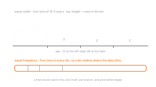
Four equal-width bins. The range runs 22 to 88, so each is 16.5 years wide, with interior edges at 38.5, 55 and 71.5. Counts: 13, 3, 2, 2.

Four equal-frequency bins. Quartile edges land at 28.75, 34.5 and 46. Counts: 5, 5, 5, 5, with widths of 6.75, 5.75, 11.5 and 42 years. The bottom covers under seven years because that's where everyone is; the top covers forty-two.

Same column, same number of bins, and one version has three bins that can't estimate anything.

Show Me the Code

1import numpy as np2
3ages: np.ndarray = np.array([22, 24, 25, 27, 28, 29, 31, 32, 33, 34,4                             35, 36, 38, 41, 44, 52, 58, 67, 74, 88], dtype=float)5
6wide_counts, wide_edges = np.histogram(ages, bins=4)     # equal width7print(wide_edges.tolist())                # -> [22.0, 38.5, 55.0, 71.5, 88.0]8print(wide_counts.tolist())               # -> [13, 3, 2, 2]  one bin holds most of the frame9
10q_edges: np.ndarray = np.percentile(ages, [0, 25, 50, 75, 100])11freq_counts, _ = np.histogram(ages, bins=q_edges)        # equal frequency12print(q_edges.tolist())                   # -> [22.0, 28.75, 34.5, 46.0, 88.0]13print(freq_counts.tolist())               # -> [5, 5, 5, 5]  same count, very different widths14
15def assign(value: float, edges: np.ndarray) -> int:16    return int(np.clip(np.digitize(value, edges[1:-1]), 0, len(edges) - 2))17
18print(assign(34.4, q_edges), assign(34.6, q_edges))      # -> 1 2  0.2 years apart, now unrelated

The last line is the boundary artefact: two ages a fifth of a year apart, in different bands.

Watch Out For

Binning a column and then handing it to a tree

KBinsDiscretizer into LGBMClassifier, or a pd.cut on age followed by XGBoost. Written constantly, and it can only lose.

The tree was already going to search that column. It scores every candidate split point against your loss and picks per node, so a deep tree can use 40 in one branch and 62 in another. You replaced that with four fixed edges chosen without ever looking at the target.

If the reason is "it reduces noise", reach for a transform instead.

Edges fitted on training data meeting a value from outside the range

Your bin edges came from a training set where age topped out at 88. A 94-year-old arrives, pd.cut returns NaN, and the row crashes or gets imputed. KBinsDiscretizer clips into the outer bin instead, worth knowing rather than discovering. Set explicit outer edges at -inf and +inf.

The other half is supervised edges. Weight-of-evidence bins and tree-derived thresholds are chosen using the target, so they're fitted state exactly like a target encoder, and computing them once makes every fold optimistic in the same direction.

The Quick Version

Binning deletes resolution deliberately. Assume it's wrong until you can name why it isn't.
A tree finds its own thresholds, per node, against your loss.
It pays for a step a linear model can't fit, a non-monotone relationship, a rule written in bands, extremes you want kept, and a feature you monitor.
Equal-width bins have equal widths and unequal counts, so skewed data gets empty top bins.
Equal-frequency bins hold the same count and get wide in the tail. Usually the right default.
Supervised binning picks edges from the target: tree thresholds, or weight of evidence.
Ordinal indices keep the order. One-hot gives each band its own effect.
An edge at 40 makes 39.9 and 40.1 unrelated, worst where the data is densest.
Supervised edges leak unless refitted per fold, and an out-of-range value becomes a NaN.