Data Concepts

Non-Linear Transformations

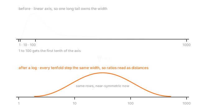
Scaling slides and stretches a distribution. A log changes its shape, and shape is what turns equal ratios into equal distances a linear model can add up.

A linear axis crushes a right-skewed column into its first tenth, and a log gives each tenfold step the same width, so the same rows come out symmetric

Why Does This Exist?

House prices from £80,000 to £4.2 million. Fit a linear model on the raw column and it commits to one number: how many pounds the price moves per extra square metre. One number, terrace and mansion alike.

That's wrong in a specific way. An extra bedroom doesn't add a flat £40,000; it adds something like 12%. Income, price, latency, population, file size: nearly everything people care about is multiplicative, so equal ratios matter.

Feature scaling can't help, because standardisation subtracts and divides and the histogram keeps its shape. A log turns ratios into differences, so a doubling adds the same amount at 100,000 as at two million.

Think of It Like This

A piano keyboard is already a log axis

Middle A vibrates at 440 Hz. The A an octave up is 880, then 1760, then 3520. In hertz the gaps keep doubling. Along the keyboard they're identical: same distance, every octave.

Nobody designed that as an arithmetic trick. Your ear hears ratios, so 440 to 880 is as big a jump as 880 to 1760, and an instrument built for hands has to space octaves evenly.

Try it the other way. Lay the keys out proportional to raw frequency and the bottom two octaves fit in a few centimetres while the top runs the length of the room, crushing every low note.

That's a right-skewed column, from a model's point of view.

How It Actually Works

Scaling is affine: multiply, then add. Affine maps preserve shape, which is why a scaled skewed column is still skewed. Everything below bends the axis instead, and bending the axis is how you change a shape.

The transforms worth knowing

Log. np.log1p computes $\log(1 + x)$ and should be your default. Plain np.log on a column holding a zero returns -inf, which doesn't raise, it propagates: it reaches your scaler and every value becomes nan.

Square root. Milder, and the natural fit for counts: a Poisson-ish count has variance equal to its mean, and $\sqrt{x}$ flattens that out.

Reciprocal. $1/x$ is aggressive and reverses the order. Right when the quantity is a rate: seconds per request into requests per second.

Box-Cox. Learns the transform instead of picking one, fitting an exponent $\lambda$ by maximum likelihood to land closest to normal. $\lambda = 1$ is no change, $0.5$ the square root, $0$ exactly the log. Positive data only.

Yeo-Johnson. Box-Cox rebuilt for zeros and negatives, a different branch each side of zero. The general-purpose pick.

Quantile transform. Ranks every value and maps the ranks onto a normal or uniform distribution, so it always works. The original spacing is gone, and it can't extrapolate past the training range.

Trees don't care

Every transform above is monotone. If x > 40 splits your rows one way, log(x) > log(40) splits them the same way, because the order didn't change and a tree only asks about order. Random forests, gradient boosting, extra trees: no effect.

So this is for linear and logistic regression, distance methods, and networks, where one heavy tail means a few rows dominate the gradient.

Transform the target and the metric moves too

Squared error on $\log y$ is not squared error on $y$ . Minimising the first minimises roughly relative error on the original scale, which is usually what you wanted: £20,000 out on a £2 million house isn't the mistake £20,000 out on a £150,000 flat is.

Coming back is where it bites. expm1 of a prediction is a median, not a mean: the average of the logs is the log of the geometric mean, which always sits below the arithmetic mean. Predictions come back low, more so the wider the residual spread. Correct it with $\exp(\hat{\sigma}^2/2)$ , or fit the original scale with a log link.

Worked example

Ten values that double each step: 1, 2, 4, 8, up to 512. The mean is $1023/10 = 102.3$ and the median is 24, so the mean beats eight of the ten values, the signature of a right tail (descriptive statistics covers why they diverge). Skewness is about 1.76.

Take $\log_2$ and the column becomes 0, 1, 2, up to 9. Symmetric, skewness exactly 0. The transform didn't tame outliers, it showed there weren't any: every gap was one doubling.

Then the round trip. The mean of the logs is 4.5, and $2^{4.5} = 22.63$ : the geometric mean, next to the median and nowhere near 102.3.

Show Me the Code

1import numpy as np2
3x: np.ndarray = 2.0 ** np.arange(10)           # [1, 2, 4, ... 512] a doubling column4
5def skew(a: np.ndarray) -> float:6    d = a - a.mean()7    return float((d ** 3).mean() / (d ** 2).mean() ** 1.5)8
9print(x.mean(), np.median(x))                   # -> 102.3 24.0  mean beats 8 of the 10 values10print(round(skew(x), 2))                        # -> 1.76  long right tail11print(round(skew(np.log2(x)), 2))               # -> 0.0   the log made it symmetric12
13print(float(np.log1p(0.0)))                     # -> 0.0   log1p absorbs the zero14with np.errstate(divide="ignore"):15    print(float(np.log(0.0)))                   # -> -inf  plain log poisons the column16
17geo: float = float(np.exp(np.log(x).mean()))    # exp of the mean of the logs18print(round(geo, 2))                            # -> 22.63  near the median 24.0, not the mean

The last line is the target-transform trap: back-transform a mean and you get 22.63, when the data's mean is 102.3.

Watch Out For

A log on a column with zeros, and a transform fitted on everything

np.log(revenue) where revenue holds a single zero, and one cell is now -inf. Nothing raises. Subtract the mean and the whole column becomes nan, and the error complains about input validation while saying nothing about logs. Default to log1p, and check np.isfinite(x).all() afterwards.

Box-Cox learns $\lambda$ from data and the quantile transform learns an entire mapping from the empirical distribution, so both are fitted state. Fit on training rows and persist the object with the model. Call fit_transform on the full frame and your validation rows helped choose the transform that scored them: data leakage.

Forgetting the target's inverse, or comparing metrics from different scales

You trained on log1p(price), so the model predicts log-pounds. Skip the expm1 and the predictions are wrong by orders of magnitude and the RMSE is in units nobody can interpret.

The subtler version shows up in write-ups: an RMSE of 0.21 on log-price set against someone else's 48,000 on price, as though the smaller number won. Log-scale error is roughly proportional error, so 0.21 is about 23% off. Pick one scale, invert before scoring, and report on the scale the decision is made in.

The Quick Version

Scaling is affine and preserves shape. These transforms bend the axis, which changes a shape.
Real positive quantities are multiplicative, and a log turns equal ratios into equal differences.
log1p is the default. Plain log on a zero gives -inf, which spreads silently.
Square root suits counts. The reciprocal suits rates and flips the order.
Box-Cox learns the exponent by maximum likelihood and needs positive data. Its zero case is the log.
Yeo-Johnson handles zeros and negatives, so it's the general-purpose choice.
A quantile transform forces any shape to normal or uniform and can't extrapolate.
Trees are unaffected: every transform here is monotone, so the splits are identical.
Back-transforming a mean prediction gives a median, so predictions come back low.
The exponent and the quantile mapping are fitted state. Fit on training rows only.