Gen AI

Scaling Laws

Model performance improves predictably as you increase compute, dataset size, and parameter count, forming a smooth power-law curve that lets researchers forecast success before spending millions on a training run.

Why Does This Exist?

Training a frontier AI model costs tens or hundreds of millions of dollars in compute time. If you are going to write a check that large to rent thousands of GPUs for six months, you cannot simply guess that the resulting model will be smart enough to justify the cost. You need a mathematically sound guarantee that the investment will yield a proportionate decrease in the model's error rate.

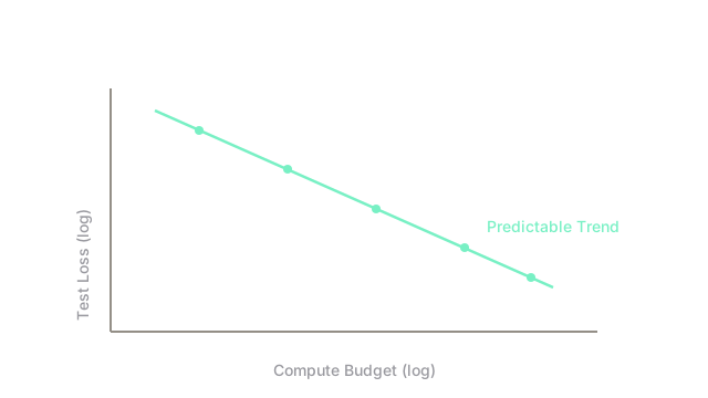
Scaling laws provide that guarantee. They are empirical observations that demonstrate a smooth, highly predictable relationship between the resources poured into an LLM (compute, data, and parameters) and the model's final performance. Because these laws hold true across many orders of magnitude, researchers can train a tiny, cheap model, measure its performance, and confidently extrapolate exactly how smart a massive, expensive model will be if built using the same architecture.

Think of It Like This

Predicting the top speed of a race car from an RC model

Imagine you are designing a new type of race car engine. Building a full-size prototype costs a fortune. But you discover a law of physics for this engine: every time you double the fuel flow and double the engine volume, the top speed reliably increases by exactly 15%.

Because you know this rule holds perfectly, you don't need to build the full-size car to know how fast it will go. You build a cheap remote-control version, measure its speed, and simply draw a line on a graph to figure out exactly how much fuel and metal you'll need to hit 200 mph in the final product. Scaling laws are the equivalent rule for neural networks.

How It Actually Works

The power-law relationship

In 2020, researchers at OpenAI published a landmark paper observing that language model performance (measured as the loss on a next-token prediction task) scales as a power law with three primary factors:

Compute (C): The total number of floating-point operations used during training.
Dataset Size (D): The total number of tokens the model was trained on.
Parameters (N): The size of the model itself.

When you plot the model's loss against any of these three factors on a log-log graph (where both the x and y axes increase by powers of 10), the result is a perfectly straight line.

The independence of architecture

One of the most surprising findings of scaling laws is that they are largely indifferent to the specific architectural tweaks of the model. Whether you use a slightly wider network, a slightly deeper network, or tweak the attention mechanism, the overarching curve dominates. The single biggest determinant of how capable a model will be is simply the total compute budget allocated to it, assuming the compute is spent optimally.

Breaking the curve: Bottlenecks

Scaling laws only hold true if you scale the resources in tandem. If you increase the model size (N) but keep the dataset size (D) fixed, the model will quickly overfit, and the smooth scaling curve will flatten out into an asymptote. The performance stops improving because the model has memorized the small dataset.

Conversely, if you increase the dataset size (D) but keep the model size (N) fixed, the model's limited parameters will lack the capacity to absorb all the information, and again, the curve flattens. To stay on the optimal scaling curve, you must scale all factors simultaneously.

Show Me the Code

While scaling laws are usually observed on massive supercomputers, the mathematical relationship itself is a simple power-law function. Here is how you might calculate the predicted loss based on a given compute budget, using hypothetical constants.

1import math2
3def predict_loss(compute_flops: float, L_infinity: float, scale_factor: float, alpha: float) -> float:4    """5    Predicts the test loss of a model given a compute budget.6    L(C) = L_infinity + (scale_factor / C^alpha)7    """8    # L_infinity is the theoretical lowest possible loss (irreducible entropy)9    # scale_factor is a constant dependent on the architecture10    # alpha dictates how steeply the loss drops as compute scales11    return L_infinity + (scale_factor / (compute_flops ** alpha))12
13# Hypothetical constants derived from fitting small experimental runs14L_inf = 1.515k = 1e816alpha = 0.0517
18# Compute budgets (e.g., 10^18, 10^20, 10^22 FLOPs)19budgets = [1e18, 1e20, 1e22]20
21for c in budgets:22    loss = predict_loss(c, L_inf, k, alpha)23    print(f"Compute: 10^{int(math.log10(c))} FLOPs -> Predicted Loss: {loss:.3f}")24    25# -> Compute: 10^18 FLOPs -> Predicted Loss: 2.75926# -> Compute: 10^20 FLOPs -> Predicted Loss: 2.50027# -> Compute: 10^22 FLOPs -> Predicted Loss: 2.294

This simple function allows researchers to map out the exact FLOP requirement to reach a desired loss threshold, assuming the training run doesn't encounter catastrophic software bugs.

Watch Out For

Assuming scaling laws predict specific capabilities

Scaling laws predict a smooth decrease in overall loss (how well the model guesses the next word on average). They do not guarantee smooth improvements in specific, narrow capabilities. The overall loss might drop predictably, but the model's ability to solve a specific math puzzle or write a specific type of code might suddenly jump from 0% accuracy to 80% accuracy in a single generation. This phenomenon is related to the concept of emergent abilities.

Running out of high-quality data

Scaling laws assume you have an infinite supply of fresh, high-quality data to feed the increasingly massive models. As models scale into the trillions of parameters, researchers are rapidly depleting the internet's supply of human-generated text. If the data quality drops (e.g., training on synthetic garbage), the scaling curve breaks, and adding more compute no longer yields the expected intelligence gains.

The Quick Version

Scaling laws demonstrate a predictable, mathematical relationship between the resources poured into an LLM and its final performance.
When plotted on a log-log scale, increasing compute, dataset size, or parameter count yields a straight-line reduction in model error.
This predictability allows researchers to test cheap, small models and confidently extrapolate the performance of massive, expensive models.
To stay on the optimal scaling curve, parameters and data must be scaled simultaneously; scaling one without the other leads to diminishing returns.