Advanced Linear Algebra for ML

A map of the decompositions that run machine learning: which factorisation to reach for, what each one costs, and which trap each one avoids.

One matrix fans out to five decompositions, each answering a different question: LU solves, QR orthogonalises, Cholesky speeds up symmetric systems, eigendecomposition finds axes, SVD ranks everything

Why Does This Exist?

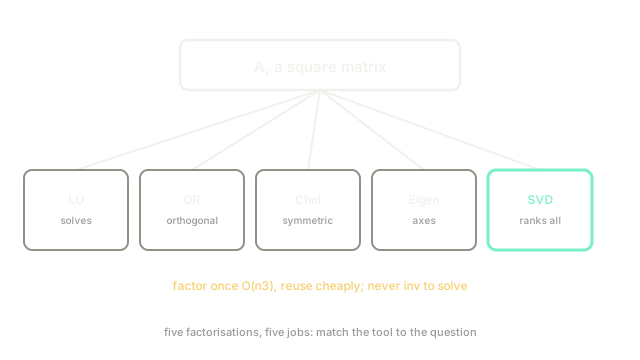
Basic linear algebra teaches you what a matrix is. Advanced linear algebra teaches you what to do with one, and the answer is almost always a decomposition: rewriting the matrix as a product of simpler pieces that expose the property you need. Solving, orthogonalising, ranking, finding axes: each job has a factorisation, each factorisation has a cost, and picking wrong costs real money at scale.

The map, in one list:

LU: $A = LU$ with triangular factors. The workhorse for square systems; factor once, solve many right-hand sides cheaply.
QR: $A = QR$ with orthonormal $Q$ . Stable least squares and every orthogonalisation routine.
Cholesky: $A = LL^T$ for symmetric positive definite matrices. Half the cost of LU; the fast path for covariances and kernels.
Eigendecomposition: $A = PDP^{-1}$ (or $Q\Lambda Q^T$ when symmetric). Axes and long-run behaviour.
SVD: $A = U\Sigma V^T$ for any shape. Ranking, compression, the pseudo-inverse that never fails.

Details live on their own pages: linear systems and least squares, singular value decomposition, eigenvalues and eigenvectors. This page is the map that says which one your problem needs.

The one idea you need first

A factorisation rewrites $A$ as a product whose pieces are easier than $A$ : triangular systems solve by substitution, orthogonal matrices invert by transposing, diagonal matrices power entry by entry. You pay once to factor, then every later operation is cheap. That pay-once structure is the economic argument behind all five entries.

Think of It Like This

A workshop wall of specialised saws

A workshop stocks five saws that all cut wood. The rip saw cuts along the grain fast, the crosscut goes across cleanly, the coping saw turns corners, the hacksaw handles metal, the chainsaw fells trees. Each is the best at one cut and a poor substitute for the others.

Decompositions are that wall. LU rips through square systems, QR crosscuts into stable orthogonal pieces, Cholesky is the lighter saw for symmetric stock, eigendecomposition follows the grain of the matrix's own axes, and SVD cuts anything including shapes the other saws cannot clamp. Reaching for the nearest saw instead of the right one is how $O(n^3)$ bills and numerically mangled answers happen.

How It Actually Works

Match the job to the tool:

Solve $Ax = b$ , square and ordinary → LU with partial pivoting ( $2n^3/3$ flops). Factor once; each new $b$ costs $O(n^2)$ .
Least squares or orthonormal basis → QR. Never form the normal equations $X^TX$ when QR on $X$ is stable and direct.
Symmetric positive definite system (covariance, kernel, Hessian near a minimum) → Cholesky ( $n^3/3$ flops, no pivoting needed). If it fails, the matrix was not positive definite and you just learned something.
Powers, exponentials, long-run behaviour → eigendecomposition, via diagonalisation when the matrix allows it.
Rank, compression, any shape, failing gracefully → SVD. The most expensive and the most informative.

Worked example

Solve a small system the right way, with substitution instead of an inverse:

\begin{bmatrix} 3 & 1 \\ 1 & 2 \end{bmatrix} \begin{bmatrix} x_1 \\ x_2 \end{bmatrix} = \begin{bmatrix} 9 \\ 8 \end{bmatrix}

Eliminate: subtract $1/3$ of row one from row two, giving $[0, 5/3]$ against $8 - 3 = 5$ . Back-substitute: $x_2 = 5 \cdot 3/5 = 3$ , then $3x_1 = 9 - 3$ so $x_1 = 2$ . Answer $x = [2, 3]$ . Check: $3 \cdot 2 + 3 = 9$ and $2 + 6 = 8$ . No inverse was formed, no determinant computed; elimination plus substitution did everything.

Code

The point is the check: solve directly and confirm the residual vanishes, instead of forming an inverse.

1import numpy as np2
3
4A = np.array([[3.0, 1.0], [1.0, 2.0]])5b = np.array([9.0, 8.0])6x = np.linalg.solve(A, b)  # LU under the hood, never an explicit inverse7print(x)                                # -> [2. 3.]8print(np.allclose(A @ x, b))            # -> True

solve factors and substitutes; inv(A) @ b inverts and multiplies, costing more while amplifying rounding error. Same answer here, different bills and different stability at scale.

Watch Out For

Calling inv when you needed solve

np.linalg.inv(A) @ b is the most common linear-algebra performance bug in ML code: three times the flops of solve, worse error bounds, and an explicit inverse nothing downstream needs. Unless the inverse matrix itself is the deliverable, factor and substitute. Linters will not catch this; only habit does.

Forming the Gram matrix before decomposing

Computing $X^TX$ squares the condition number: a mildly ill-conditioned $X$ becomes a hopelessly ill-conditioned $X^TX$ , and information is destroyed before the solver starts. Factor $X$ directly (QR for least squares, SVD for the full picture) and leave the Gram matrix unforged.

The Quick Version

Advanced linear algebra is choosing decompositions: LU solves, QR orthogonalises, Cholesky speeds symmetric cases, eigendecomposition finds axes, SVD ranks anything.
Factor once at $O(n^3)$ , then solve each new right-hand side at $O(n^2)$ .
The 2-by-2 system above solves to $x = [2, 3]$ by elimination, no inverse involved.
Never call inv to solve a system; never form $X^TX$ when QR or SVD on $X$ works.
Cholesky failing is a diagnosis: the matrix was not positive definite.