Math

Linear Systems and Least Squares

When there is no exact answer, settle for the closest one — and the closest one has a property so specific it hands you a formula.

When no line passes through every point, least squares picks the one whose leftover errors are perpendicular to everything the model could have fitted, which forces the residuals to cancel out

Why Does This Exist?

Linear regression has a closed-form solution. Not an approximation, not an iterative procedure — an exact formula that lands on the best possible answer in one step. This page derives it, and the derivation explains most of what people find confusing about regression afterwards.

Three things fall out of it.

Where the formula comes from. $\hat{\beta} = (X^{T}X)^{-1}X^{T}y$ is not something to memorise. It is what you get from one geometric idea, and once you see the idea the formula is obvious.

Why nobody uses it at scale. Inverting $X^{T}X$ costs $O(d^3)$ and squares the condition number, which is why gradient descent wins on large problems despite being iterative and approximate. That is a genuine engineering trade, not laziness.

Why correlated features break it. Multicollinearity is not a vague warning — it is the matrix $X^{T}X$ becoming singular, and ridge regression is the specific repair. Both are visible in the algebra.

This is the mathematics only. How the model is fitted in practice, its assumptions, and what its residuals tell you belong to linear regression as a model; here we derive the solution.

Think of It Like This

The closest point on a road you cannot leave

You are standing in a field and you want to reach a friend who is confined to a straight road. You cannot bring them off the road, so you settle for the closest point on it.

Where is that point? Walk perpendicular to the road. Any other choice leaves you further away — this is the one direction that gives up nothing. And the give-away signature of having arrived is that the line from your friend's position back to you is at right angles to the road.

Least squares is that, with the road being everything your model is capable of predicting. Your data $y$ is out in the field, unreachable. The set of achievable predictions is a flat surface — a line, a plane, a higher-dimensional version — and the best available prediction is the perpendicular drop onto it.

The right-angle condition is the whole thing. It is not a description of the answer, it is a test the answer must satisfy, and turning that test into algebra produces the formula.

How It Actually Works

A linear system $Ax = b$ has three possible situations, and it is worth naming them before solving anything:

Exactly one solution — $A$ is square and full rank. Rare with real data.
No solution — more equations than unknowns, and $b$ does not lie in the reachable set. This is the normal case in ML: more data points than parameters. This is what least squares is for.
Infinitely many — fewer independent equations than unknowns. Then you need a rule for choosing, and the usual one is minimum norm.

Setting up the problem

With $X \in \mathbb{R}^{n \times d}$ ( $n$ examples, $d$ features) and targets $y \in \mathbb{R}^{n}$ , we cannot generally solve $X\beta = y$ . So minimise the squared error instead:

\hat\beta = \arg\min_\beta \lVert y - X\beta \rVert_2^2

In plain words: choose the coefficients making the total squared miss as small as possible. Squaring is not arbitrary — it comes from assuming Gaussian errors, which maximum likelihood estimation shows produces exactly this objective.

The normal equations, from the right angle

The set of achievable predictions $\{X\beta\}$ is the column space of $X$ . The residual $r = y - X\hat\beta$ must be perpendicular to it, which means perpendicular to every column of $X$ :

X^{T}(y - X\hat\beta) = 0

In plain words: every feature's dot product with the leftover error is zero — no feature has any remaining explanatory power. Expanding gives the normal equations:

X^{T}X\,\hat\beta = X^{T}y

and when $X^{T}X$ is invertible:

\hat\beta = (X^{T}X)^{-1}X^{T}y

That is the closed form, derived in three lines from one geometric condition. You can also reach it by setting the gradient of the loss to zero and it agrees, which is a good consistency check.

$X^{T}X$ is symmetric and positive semi-definite by construction, and it is positive definite exactly when $X$ has full column rank. That condition is the whole story of when the formula works.

Two consequences worth knowing

Residuals sum to zero whenever there is an intercept. The intercept is a column of ones, and orthogonality to it says $\sum_i r_i = 0$ . So if your residuals do not sum to zero, either you have no intercept or you have a bug.

The hat matrix is a projection. $\hat y = X\hat\beta = X(X^{T}X)^{-1}X^{T}y = Hy$ , and $H$ satisfies $H^2 = H$ — projecting twice changes nothing, which is what "projection" means. Its trace equals the number of parameters, which is where degrees of freedom come from.

Why the closed form loses at scale

Three reasons, and all three matter:

Cost. Forming $X^{T}X$ is $O(nd^2)$ and inverting it is $O(d^3)$ . At $d = 10^6$ that is $10^{18}$ operations, and the matrix alone would need 4 TB.
Conditioning. $\kappa(X^{T}X) = \kappa(X)^2$ . Squaring the condition number squares your numerical error, so a moderately awkward $X$ becomes a badly behaved $X^{T}X$ .
It only exists for this loss. Change to absolute error, add a nonlinearity, or use any other model and there is no formula at all. Gradient descent does not care.

The right answer numerically is never to invert. np.linalg.lstsq uses SVD and computes the pseudo-inverse $X^{+} = V\Sigma^{+}U^{T}$ , which works even when $X^{T}X$ is singular and picks the minimum-norm solution among the ties.

Worked example

Fit $y = mx + c$ through three points: $(1, 1)$ , $(2, 4)$ , $(3, 4)$ .

Build the design matrix with a column of ones for the intercept:

X = \begin{bmatrix} 1 & 1 \\ 2 & 1 \\ 3 & 1 \end{bmatrix}, \qquad y = \begin{bmatrix} 1 \\ 4 \\ 4 \end{bmatrix}

Then $X^{T}X = \begin{bmatrix} 14 & 6 \\ 6 & 3 \end{bmatrix}$ and $X^{T}y = \begin{bmatrix} 21 \\ 9 \end{bmatrix}$ . Check the first entry by hand: $1{\cdot}1 + 2{\cdot}4 + 3{\cdot}4 = 21$ ✓.

The determinant is $14 \times 3 - 36 = 6$ , so:

\hat\beta = \frac{1}{6}\begin{bmatrix} 3 & -6 \\ -6 & 14 \end{bmatrix}\begin{bmatrix} 21 \\ 9 \end{bmatrix} = \frac{1}{6}\begin{bmatrix} 63 - 54 \\ -126 + 126 \end{bmatrix} = \begin{bmatrix} 1.5 \\ 0 \end{bmatrix}

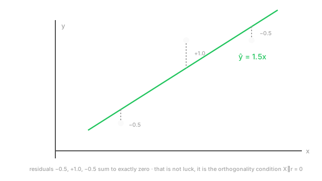
So $m = 1.5$ and $c = 0$ exactly — the fitted line is $\hat y = 1.5x$ .

Predictions are $1.5$ , $3$ , $4.5$ , giving residuals $-0.5$ , $+1.0$ , $-0.5$ . They sum to zero, as the intercept column guarantees. Squared error is $0.25 + 1 + 0.25 = 1.5$ .

Now verify the orthogonality condition that produced the whole formula:

X^{T}r = \begin{bmatrix} 1{\cdot}(-0.5) + 2{\cdot}1 + 3{\cdot}(-0.5) \\ -0.5 + 1 - 0.5 \end{bmatrix} = \begin{bmatrix} -0.5 + 2 - 1.5 \\ 0 \end{bmatrix} = \begin{bmatrix} 0 \\ 0 \end{bmatrix}

Both zero. The residual really is perpendicular to both columns, which is the geometric statement the diagram draws.

Show Me the Code

1import numpy as np2
3X = np.array([[1.0, 1.0], [2.0, 1.0], [3.0, 1.0]])   # (3, 2): slope col, intercept col4y = np.array([1.0, 4.0, 4.0])                         # (3,)5
6beta = np.linalg.lstsq(X, y, rcond=None)[0]           # SVD-based, never inverts7print(np.round(beta, 6).tolist())                     # -> [1.5, 0.0]8
9r = y - X @ beta                                       # residuals, shape (3,)10print(np.round(r, 6).tolist())                        # -> [-0.5, 1.0, -0.5]11print(round(float(r.sum()), 10))                       # -> 0.0   intercept forces this12print(np.round(X.T @ r, 10).tolist())                  # -> [0.0, 0.0]  orthogonality13print(round(float(r @ r), 6))                          # -> 1.5   squared error14
15# The normal equations agree here, and square the condition number doing it.16print(np.round(np.linalg.solve(X.T @ X, X.T @ y), 6).tolist())         # -> [1.5, 0.0]17print(round(np.linalg.cond(X), 3), round(np.linalg.cond(X.T @ X), 3))  # -> 5.331 28.42

Every number matches the hand calculation. The last line is the conditioning argument made concrete: 5.3 becomes 28.4, and that squaring is exactly why lstsq is preferred.

Watch Out For

Inverting X-transpose-X instead of using a least-squares solver

np.linalg.inv(X.T @ X) @ X.T @ y transcribes the textbook formula and is the wrong way to compute it, for two separate reasons.

The first is conditioning. Forming $X^{T}X$ squares the condition number, so you enter the solve with double the relative error you started with. With mildly correlated features — which is most real data — that is the difference between four reliable digits and none.

The second is failure mode. If any feature is an exact combination of others, $X^{T}X$ is singular and inv either raises or, worse, returns garbage full of enormous cancelling values. The classic trigger is the dummy-variable trap: one-hot encoding every level of a category and keeping an intercept makes the columns sum to the intercept column exactly.

np.linalg.lstsq avoids both. It works from the SVD, never forms $X^{T}X$ , tolerates rank deficiency, and returns the minimum-norm solution when the answer is not unique. It also reports the rank, which is free diagnostic information. There is no case where the hand-rolled inverse is better — use the solver.

Reading coefficients from an ill-conditioned fit

When features are nearly collinear the fit is still computable and the coefficients become meaningless.

The mechanism: if two features are almost identical, then many coefficient pairs produce nearly the same predictions — a large positive weight on one and a large negative weight on the other cancels out. Least squares picks one of those arbitrarily, driven by noise. So you get huge coefficients of opposite sign, excellent training fit, and a model that swings violently on new data because the cancellation no longer holds exactly.

The tell is instability rather than error. Refit on a bootstrap resample and the coefficients change substantially, sometimes flipping sign. If you are interpreting coefficients — "this feature contributes +3.2" — that interpretation is worthless here, and no amount of statistical significance testing rescues it, because the standard errors are inflated too.

Check the condition number of $X$ before trusting coefficients; above roughly $10^{3}$ treat them as unreliable, and check variance inflation factors per feature. The fixes are to drop or combine the redundant features, or to add ridge regularisation, which replaces $X^{T}X$ with $X^{T}X + \lambda I$ — guaranteed positive definite, so it is always invertible, and it shrinks the cancelling pairs toward each other. That is why ridge is the default for wide correlated data.

The Quick Version

A linear system has one solution, none, or infinitely many. With more data than parameters, "none" is normal — hence least squares.
Minimise $\lVert y - X\beta \rVert_2^2$ . The squaring comes from assuming Gaussian errors, via maximum likelihood.
The best prediction is the orthogonal projection of $y$ onto the column space of $X$ .
The right-angle condition $X^{T}(y - X\hat\beta) = 0$ is what produces the normal equations $X^{T}X\hat\beta = X^{T}y$ .
Closed form: $\hat\beta = (X^{T}X)^{-1}X^{T}y$ , valid exactly when $X$ has full column rank.
With an intercept, residuals sum to zero. If yours do not, something is wrong.
$\hat y = Hy$ where $H$ is a projection: $H^2 = H$ , and $\text{trace}(H)$ is the parameter count.
Do not use it at scale: $O(d^3)$ to invert, it squares the condition number, and it only exists for this one loss.
Use np.linalg.lstsq — SVD-based, rank-deficiency tolerant, minimum-norm.
Collinear features make coefficients unstable and uninterpretable. Ridge adds $\lambda I$ and guarantees invertibility.