Differential Equations Systems

Equations that say how things change become flows: follow the arrows and you get trajectories, equilibria, and the long-run fate of the system.

A decaying flow from 3 toward 0 shows trajectories following vector-field arrows into a stable equilibrium

Why Does This Exist?

Machine learning trains by flows (gradient descent is a discretized flow), samples by flows (diffusion reverses a stochastic one), and models time with flows (neural ODEs integrate one). Each case asks the same dynamical questions: where does motion stop, which stops attract, how fast, and what discretization breaks. Differential equations write the local rule; dynamical systems study the global fate: equilibria, stability, cycles, and bifurcations. This page maps that territory. The rule families get their own pages for ODEs and PDEs; equilibria, portraits, stability, and solvers follow as siblings. Vector-field language is in vector fields.

The one idea you need first

$\dot{x} = f(x)$ assigns every state an arrow $f(x)$ . A trajectory $x(t)$ follows the arrows: $x(t)$ moves where the field points, fast where arrows are long. Fixed points sit where $f = 0$ ; everything else is transit.

Think of It Like This

A landscape of streams after rain

Rain on hills runs downhill everywhere at once: each puddle's path follows the local slope, rivulets merge in valleys, and lakes sit where no slope remains. The slope rule is the differential equation; the full pattern of streams and lakes is the dynamical system.

A lake that pulls nearby water in is a stable equilibrium; a ridge crest shedding water both ways is unstable; a mountain pass is a saddle. Changing the landscape slowly can create or destroy lakes (bifurcation), and stepping downhill in big jumps can overshoot the lake entirely (what bad solvers do).

Where the analogy stops: real state spaces have many dimensions with cycles and chaos that no hillside shows, and stochastic systems add diffusion to the drift.

How It Actually Works

Rules. ODEs evolve finite states ( $d$ variables, $d$ arrows). PDEs evolve fields (temperature at every point). Stochastic differential equations add noise to the drift. Delay and discrete maps change the clock.

Fates. Fixed points ( $f = 0$ ), limit cycles (isolated closed orbits), attractors (sets that pull neighbours), basins (who drains where), bifurcations (qualitative change under parameters). Chaos is bounded aperiodic motion with sensitive dependence: same rules, unpredictable addresses.

Analyses. Linearize at equilibria and read Jacobian eigenvalues (stability); draw or compute portraits and nullclines (geometry); integrate numerically with step control (simulation); study conservation and Lyapunov functions (certificates).

Worked example

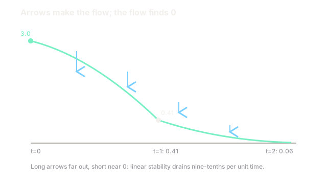
Decay $\dot{x} = -2x$ from $x(0) = 3$ . Solution $x(t) = 3e^{-2t}$ : at $t = 1$ , $x = 3e^{-2} \approx 3(0.1353) \approx 0.406$ . Fixed point $0$ (where $-2x = 0$ ), linearization $-2 < 0$ , so stable: every start drains to it, fast early (arrow $-6$ at $x = 3$ ) and slow near (arrow $-0.8$ at $x = 0.4$ ). Double time to $t = 2$ and $x \approx 0.055$ : nine-tenths of the remaining distance drains per unit time, the signature of linear stability.

Watch Out For

Assuming solutions exist, stay unique, and follow the picture

With rough $f$ (square roots, absolute values, switches), trajectories can branch, merge, or refuse to start: uniqueness needs Lipschitz continuity, and existence needs tamer growth than textbooks admit. Filippov and hybrid machinery exists precisely because ML controllers switch.

Symptom: solvers disagree qualitatively (one sticks at zero, another leaves), or adaptive steppers shrink to zero near a kink. Fix: check Lipschitz at equilibria and switches, smooth or regularize the kink, and distrust any portrait drawn through a non-Lipschitz point.

Confusing the flow with its discretization

The ODE can be stable while Euler with a big step oscillates or explodes: stability regions belong to the method, not the equation. Stiff systems (fast and slow modes together) punish explicit steppers hardest.

Symptom: shrinking the step flips the answer from blow-up to calm, or implicit methods succeed where explicit ones die at any step. Fix: match the solver to stiffness (implicit or exponential integrators), respect step bounds from the fastest mode, and test refinement before believing any simulated fate.

The Quick Version

Differential equations write local arrows; dynamical systems study where following them leads.
Fates include fixed points, cycles, attractors, basins, bifurcations, and chaos.
Decay from 3 under $\dot{x} = -2x$ reaches 0.41 at $t = 1$ toward the stable point 0.
Existence and uniqueness need Lipschitz rules; switches break naive pictures.
Discretization has its own stability: match the solver to stiffness and refine.