Ordinary Differential Equations

One clock, finitely many variables, and a rule for velocities: ODEs turn "how fast is each thing changing right now" into full trajectories.

The solution starting at 0 climbs toward its steady state 4, reaching 2.53 by time 2 along the velocity arrows

Why Does This Exist?

Motion, growth, cooling, charging, and gradient flows all say how fast: velocity as a function of position and time. An ODE is that statement plus a starting point, and its solution is the whole future. Closed forms exist for a precious few (linear, separable, exact); everything else needs qualitative analysis or numerics. Neural ODEs, diffusion samplers, and continuous optimizers all integrate ODEs at scale, so the vocabulary of order, linearity, initial values, and steady states pays off far beyond the classroom. Integration technique is in definite and indefinite integrals; stepping rules get their own solver page.

The one idea you need first

$\dot{x} = f(x, t)$ with $x(0) = x_0$ asks for the curve through $x_0$ whose slope at each instant equals $f$ . Order is the highest derivative present; linear means $f$ is affine in $x$ ; autonomous means no explicit $t$ .

Think of It Like This

A speedometer wired to the odometer

A car's speedometer is rigged to show speed based on the odometer reading and the clock: at mile $x$ and time $t$ , drive at $f(x, t)$ miles per hour. Start at mile 0 at noon and just obey: the odometer traces one curve, fully determined by the wiring and the start.

Linear wiring (speed proportional to distance remaining) glides into the destination. A steady state is the mile where the dial reads zero: arrive and stop. Stiff wiring (violent corrections plus gentle drift) makes obeying with glances every minute overshoot wildly, which is why solvers care about stiffness.

Where the analogy stops: real ODEs couple many variables with their own wirings, and existence needs the wiring to not jump discontinuously.

How It Actually Works

First-order linear. $\dot{x} + p(t)x = q(t)$ falls to integrating factors: multiply by $\mu = \exp(\int p)$ and the left becomes a total derivative. Constant-coefficient $\dot{x} = ax + b$ solves to $x(t) = (x_0 + b/a)e^{at} - b/a$ for $a \ne 0$ : exponential approach to $-b/a$ when $a < 0$ .

Separable and exact. $\dot{x} = g(x)h(t)$ splits as $dx/g(x) = h(t)dt$ and integrates each side. Exact equations hide a potential whose level sets are solutions.

Systems and higher order. $\dot{\mathbf{x}} = A\mathbf{x}$ exponentiates the matrix; $n$ th-order linear ODEs become first-order systems in $n$ variables. Nonlinear systems linearize at equilibria for local stability.

Worked example

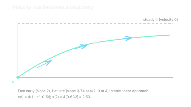
$\dot{x} = -0.5x + 2$ with $x(0) = 0$ . Steady state where $-0.5x + 2 = 0$ : $x^* = 4$ . With $a = -0.5$ , $b = 2$ :

x(t) = 4(1 - e^{-0.5t})

At $t = 2$ : $e^{-1} \approx 0.3679$ , so $x(2) = 4(1 - 0.3679) = 4(0.6321) \approx 2.528$ . Velocity starts at $2$ (full throttle from 0), falls to $-0.5(2.528) + 2 \approx 0.736$ by $t = 2$ , and vanishes at 4: the curve climbs fast then flattens, the universal shape of stable linear approach.

Watch Out For

Expecting closed forms where none exist

Most nonlinear ODEs (pendulum at large angles, three-body, Lorenz) have no elementary solution: the integral that "solves" them is not expressible, and series or special functions only rename the difficulty. Time spent hunting a formula is time not spent on portraits or numerics.

Symptom: pages of substitutions circling back to the start equation. Fix: linearize for local behaviour, draw the phase line or portrait for global shape, and integrate numerically for numbers. Reserve analytic effort for linear, separable, and exact cases.

Ignoring stiffness when stepping

Decaying modes with rates $1$ and $1000$ force explicit steppers down to the fast scale even after the fast transient dies: steps of $1/1000$ to track a curve that barely moves. Any bigger step oscillates or explodes while the true solution sits calm.

Symptom: Euler or RK4 needs absurdly many steps on a smooth-looking problem, or blows up at innocent step sizes. Fix: detect stiffness (separated Jacobian eigenvalues with large negative real parts) and switch to implicit or exponential methods, as the solver page details.

The Quick Version

ODEs solve velocity rules from starting values into trajectories.
Linear constant-coefficient equations approach $-b/a$ exponentially when $a < 0$ .
The worked equation climbs from 0 to 2.53 by $t = 2$ toward steady state 4.
Most nonlinear ODEs need geometry or numerics, not formulas.
Stiff systems demand implicit steppers; explicit ones crawl or blow up.