Symmetric Eigendecomposition

A symmetric matrix is a stretch along perpendicular axes, no rotation mixed in. Its eigendecomposition names those axes and the stretch on each.

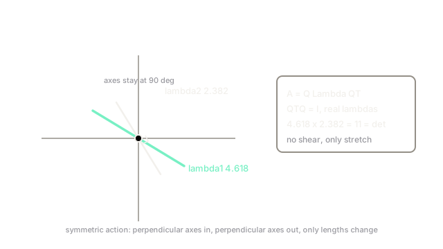
The symmetric 4 1 1 3 matrix stretches its two perpendicular eigenvector axes by 4.618 and 2.382, with no rotation mixed in

Why Does This Exist?

Covariance matrices, Hessians, kernels and graph Laplacians share one property: symmetry ( $A^T = A$ ). Symmetry buys the strongest decomposition in linear algebra. Where a general matrix needs a fragile $PDP^{-1}$ with an explicit inverse, a symmetric matrix splits into $A = Q\Lambda Q^T$ with $Q$ orthogonal, so the "inverse" is a free transpose. Eigenvalues come out real, eigenvectors out mutually perpendicular, and nothing can go complex or defective on you.

That is why PCA works on the covariance without fear, why the Hessian's curvature directions are trustworthy, and why spectral clustering leans on the Laplacian. General eigenvalues and eigenvectors teach the objects; diagonalisation assembles them for ordinary matrices. This page is the symmetric upgrade where everything becomes orthonormal.

The one idea you need first

An orthogonal matrix $Q$ satisfies $Q^T Q = I$ : its columns are unit length and mutually perpendicular, and $Q^{-1} = Q^T$ . Rotations and reflections qualify. Multiplying by $Q$ never stretches anything, it only re-views, which is why the symmetric decomposition is numerically bulletproof.

Think of It Like This

Stretching a printed grid along its own weave

Print a square grid on rubber and pin it at two perpendicular weave directions. Pull one direction harder than the other. The grid lines stay perpendicular throughout: each line keeps its direction and only changes length.

That is symmetric action. A general matrix would also shear the grid, tilting lines so they stop being perpendicular, and unpicking shear from stretch takes the fragile general machinery. Symmetry forbids shear from the start, so the matrix is fully described by "which perpendicular directions" plus "how much stretch each". Those are the eigenvectors and eigenvalues, and $Q\Lambda Q^T$ is the recipe: rotate to the weave, stretch, rotate back.

How It Actually Works

For symmetric $A$ , there exist orthonormal $q_1, \ldots, q_n$ and real $\lambda_i$ with:

A = Q\Lambda Q^T = \sum_{i=1}^n \lambda_i q_i q_i^T

Read it right to left on a vector $x$ : $Q^T$ re-views $x$ in the eigenbasis, $\Lambda$ stretches each coordinate by $\lambda_i$ , $Q$ rotates back. The sum form says $A$ is a weighted stack of rank-one projections, weight $\lambda_i$ on direction $q_i$ . Dropping small- $\lambda_i$ terms is exactly truncated PCA, and the spectral theorem states why this always works.

Worked example

Split $A = \begin{bmatrix} 4 & 1 \\ 1 & 3 \end{bmatrix}$ . Trace 7, determinant $12 - 1 = 11$ , so the characteristic equation $\lambda^2 - 7\lambda + 11 = 0$ gives:

\lambda = \frac{7 \pm \sqrt{49 - 44}}{2} = \frac{7 \pm \sqrt{5}}{2} \approx 4.618,\ 2.382

Both real, as symmetry guarantees. Their product $4.618 \times 2.382 \approx 11.0$ recovers the determinant. For $\lambda_1 \approx 4.618$ , solving $(A - \lambda_1 I)v = 0$ gives $v_1 \propto [1, 0.618]$ ; for $\lambda_2$ , $v_2 \propto [-0.618, 1]$ . Dot product: $-0.618 + 0.618 = 0$ . Perpendicular, exactly as promised, with no arrangement needed.

Code

The point is the check: reconstruct from the factors and confirm orthonormality, with no explicit inverse anywhere.

1import numpy as np2
3
4A = np.array([[4.0, 1.0], [1.0, 3.0]])5w, Q = np.linalg.eigh(A)  # symmetric solver: orthonormal Q guaranteed6print(np.allclose(Q @ np.diag(w) @ Q.T, A))  # -> True7print(np.allclose(Q.T @ Q, np.eye(2)))       # -> True

eigh (the symmetric solver) returns real eigenvalues and orthonormal vectors by construction. The general eig would work here too but promises less; on symmetric input, always reach for eigh.

Watch Out For

Assuming any diagonalisation is orthogonal

$A = PDP^{-1}$ for a general matrix has no orthogonality: $P$ 's columns can be nearly parallel, and then $P^{-1}$ amplifies rounding error catastrophically. Orthogonal diagonalisation is a symmetric privilege. Check $A^T = A$ (up to rounding) before treating an eigenbasis as orthonormal, especially for Hessians assembled by autodiff.

Depending on eigenvector signs

If $v$ is an eigenvector so is $-v$ , and solvers return either sign unpredictably across versions and machines. Code that compares eigenvectors elementwise, or plots loadings assuming a fixed orientation, breaks on upgrade. Compare subspaces (absolute values, projections, outer products $vv^T$ ) instead of raw vectors.

The Quick Version

Symmetric matrices split into $Q\Lambda Q^T$ with real eigenvalues and perpendicular eigenvectors.
The 4-1-1-3 example gives eigenvalues 4.618 and 2.382 with orthogonal axes.
The sum form shows $A$ as stacked rank-one projections, which is what PCA truncates.
Use eigh, not eig, on symmetric input: orthonormality comes guaranteed.
Eigenvector signs are arbitrary; compare subspaces, never raw vectors.