Exponential Family Distributions

Many famous distributions share one algebraic shape. Learn that shape once and Bernoulli, Poisson, and Gaussian all run on the same estimation engine.

Bernoulli, Poisson, and Gaussian each factor into base measure, sufficient statistic, and log-partition, so one convex engine fits all three

Why Does This Exist?

GLMs, conjugate priors, and variational inference all reuse the same trick: write the density as $p(x \\mid \\eta) = h(x)\\exp(\\eta^\\top T(x) - A(\\eta))$ and everything downstream becomes mechanical. Means come from $\\nabla A$ , variances from $\\nabla^2 A$ , MLE matches moments, and conjugate priors multiply cleanly.

Without the shared form, each distribution needs bespoke algebra. With it, one proof covers Bernoulli flips, Poisson counts, and Gaussian noise. It generalizes probability distributions into a working toolkit for maximum likelihood estimation.

The one idea you need first

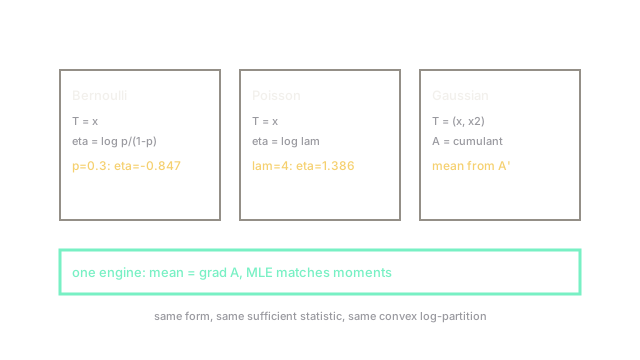
$T(x)$ is the sufficient statistic, $\\eta$ the natural parameter, $A(\\eta)$ the log-partition that normalizes. For Bernoulli with mean $p$ : $\\eta = \\log(p/(1-p))$ and $A(\\eta) = \\log(1 + e^\\eta)$ .

Think of It Like This

One charger for many phones

Bernoulli, Poisson, and Gaussian look like different phones with different ports. The exponential family is the discovery that all three charge over USB-C: same $h$ , $T$ , $\\eta$ , $A$ pins in different positions.

One charger (moment matching, convex $A$ , conjugate updates) powers all of them. Where it stops: some phones need proprietary voltage. Uniform, Cauchy, and mixture models sit outside the family and the charger does not fit.

How It Actually Works

Members share: base measure $h(x)$ , sufficient statistic $T(x)$ , natural parameter $\\eta$ , log-partition $A(\\eta) = \\log \\int h(x) e^{\\eta^\\top T(x)} dx$ . Then $\\mathbb{E}[T(X)] = \\nabla A(\\eta)$ and $\\mathrm{Cov}[T(X)] = \\nabla^2 A(\\eta)$ , with $A$ convex. MLE sets sample moments of $T$ equal to $\\nabla A(\\eta)$ , a convex problem with one global optimum in $\\eta$ .

Worked example

Bernoulli $p = 0.3$ : $\\eta = \\log(0.3/0.7) = \\log(0.4286) \\approx -0.8473$ . $A(\\eta) = \\log(1 + e^{-0.8473}) = \\log(1.4286) \\approx 0.3567$ . Derivative check: $A'(\\eta) = e^\\eta/(1+e^\\eta) = 0.4286/1.4286 = 0.3$ , the mean. Poisson $\\lambda = 4$ : $\\eta = \\log 4 \\approx 1.3863$ , $A(\\eta) = e^\\eta = 4$ , and $A' = 4$ , again the mean. Same differentiation, two distributions.

Code

1import numpy as np2
3p = 0.34eta = float(np.log(p / (1 - p)))  # natural parameter5mean = float(np.exp(eta) / (1 + np.exp(eta)))  # grad A6print(round(eta, 4), round(mean, 4))  # -> (-0.8473, 0.3)

The round trip recovers 0.3 from $-0.8473$ . Moment matching inverts $\\nabla A$ the same way for every member.

Watch Out For

Forcing outsiders into the family

Uniform on $[0, \\theta]$ has support depending on the parameter, so no fixed $h(x)$ works. Cauchy has no mean, so $\\nabla A$ cannot exist. Fitting family machinery anyway gives silently wrong posteriors and "convex" losses with kinks.

Checklist: fixed support, finite $A(\\eta)$ , and sufficient statistic of fixed dimension. Mixtures fail the last one.

Optimizing the wrong parameterization non-convexly

$A(\\eta)$ is convex in $\\eta$ , not necessarily in the everyday parameter like $p$ or $\\sigma$ . Running gradient descent on $p$ near the boundary 0 or 1 crawls or diverges, while $\\eta$ space is smooth and unconstrained.

Optimize in $\\eta$ (logits, log-rates), then map back. If the loss looks non-convex, suspect the parameterization first.

The Quick Version

One form $h(x)\\exp(\\eta^\\top T(x) - A(\\eta))$ covers Bernoulli, Poisson, Gaussian, gamma, and more.
Means and covariances are derivatives of $A$ ; $A$ is convex in $\\eta$ .
Bernoulli $p=0.3$ gives $\\eta \\approx -0.847$ and recovers the mean by differentiating.
MLE becomes moment matching with a unique optimum in natural parameters.
Uniform, Cauchy, and mixtures sit outside; check support and statistic dimension first.
Optimize in $\\eta$ , not in bounded everyday parameters.