Math

Probability Distributions

A fixed budget of belief spread across every outcome that could happen — and the shape you assume it takes is what silently decides your loss function.

A distribution hands out a fixed budget of belief across every possible outcome, and the one rule that makes it a distribution is that the budget totals exactly one

Why Does This Exist?

Here is a fact that surprises most people the first time they meet it: you never actually chose your loss function. You chose a distribution, and the loss followed from it.

Predicting a real number and using mean squared error? You assumed your errors are Gaussian. Binary classification with binary cross-entropy? You assumed a Bernoulli. Multi-class with softmax and cross-entropy? A categorical. In every case the loss is the negative log-likelihood of that assumed distribution, and reaching for it "because that is what people use for regression" means running an assumption you never inspected.

That matters because the assumptions fail in identifiable ways. Gaussian errors are symmetric with thin tails, so MSE on data with genuine outliers spends the model's capacity chasing them. Count data is not Gaussian, and forcing it to be produces a model that happily predicts negative counts. Knowing which distribution you have assumed tells you what your loss is bad at, before it embarrasses you.

Think of It Like This

One kilogram of clay

You have exactly one kilogram of clay and a row of buckets, one per possible outcome. Distributing the clay is what a distribution does. You can pile most of it into one bucket, spread it evenly, or anything between — but you always use all of it and never more than all of it.

That constraint is the whole definition, and it explains something people find odd about softmax: raising one class's probability must lower the others. Not because the classes interact in the world, but because there is only one kilogram of clay and you took some from somewhere.

Now the continuous case, which is where intuition usually breaks. If the outcomes form a continuum — any real number — you have infinitely many buckets, so the clay in any single one is zero. What you can still ask is how thickly the clay is spread at a point, and how much sits in a stretch. That thickness is a density, and it is why the probability that a continuous variable equals exactly 3.0 is zero while the probability it lands between 2.9 and 3.1 is not.

How It Actually Works

Split by whether the outcomes are countable.

Discrete distributions use a probability mass function, which gives a real probability to each outcome. Two rules, and that is all:

P(x_i) \ge 0 \quad \text{for every } i, \qquad \sum_i P(x_i) = 1

In plain words: no negative beliefs, and everything you believe adds up to exactly one.

Continuous distributions use a probability density $p(x)$ , where the same two rules hold with an integral instead of a sum:

p(x) \ge 0, \qquad \int_{-\infty}^{\infty} p(x)\, dx = 1

In plain words: total area under the curve is one. The critical difference is that $p(x)$ is not a probability and can exceed 1 — a narrow spike has to be tall to enclose area 1. Only areas are probabilities here, which is why $P(X = 3.0) = 0$ for any continuous variable.

The three you actually need

Nearly all supervised learning uses one of three, and each one maps to a loss:

Bernoulli — one yes/no outcome with probability $p$ of yes. The distribution behind binary classification, and its negative log-likelihood is binary cross-entropy.
Categorical — one outcome from $k$ classes, with probabilities summing to 1. The distribution a softmax layer produces, and its negative log-likelihood is cross-entropy.
Gaussian (normal) — a continuous bell centred at $\mu$ with spread $\sigma$ . Assumed for regression errors, and its negative log-likelihood is, up to constants, mean squared error.

That last line is worth restating because it is the most useful thing on this page: MSE is the Gaussian assumption written as code. The squared term in MSE comes directly from the squared term in the Gaussian's exponent. If you have ever wondered why regression squares its errors rather than using absolute values, that is the answer — and using absolute error instead is equivalent to assuming a Laplace distribution, which has fatter tails and is therefore more robust to outliers.

Joint, marginal, conditional

Three words that describe relationships between distributions, and they come up constantly:

Joint $P(x, y)$ — the probability of both together.
Marginal $P(x)$ — the probability of $x$ regardless of $y$ , obtained by summing the joint over every value of $y$ .
Conditional $P(y \mid x)$ — the probability of $y$ given that $x$ is known.

Supervised learning is the business of modelling $P(y \mid x)$ : the distribution over labels given an input. A classifier does not output a label, it outputs a conditional distribution, and picking the highest-probability class is a separate decision made afterwards.

Worked example

Take a biased coin with a 0.3 chance of heads — a Bernoulli with $p = 0.3$ . Encode heads as 1 and tails as 0.

The expected value is the probability-weighted average of the outcomes:

E[X] = (1 \times 0.3) + (0 \times 0.7) = 0.3

In plain words: over many flips, the average of the 1s and 0s converges to 0.3. Note the expected value is 0.3, which is not an outcome the coin can ever produce — expectations need not be attainable.

The variance for a Bernoulli works out to $p(1-p)$ :

\text{Var}(X) = 0.3 \times 0.7 = 0.21

That formula peaks at $p = 0.5$ , where variance is 0.25. A fair coin is the most unpredictable one, which is the same fact entropy measures in different units.

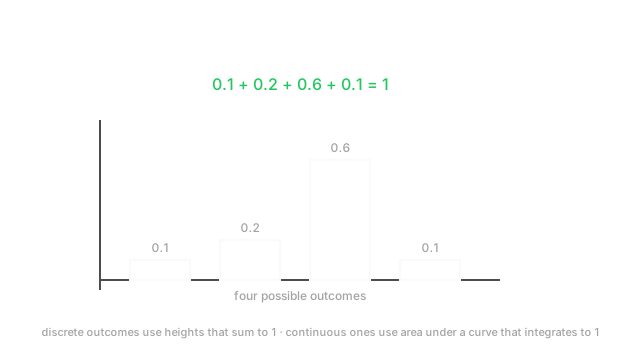
Now a categorical example, matching the diagram: four classes with probabilities $[0.1, 0.2, 0.6, 0.1]$ . They sum to 1, so it is a valid distribution. If class 3 is correct, the cross-entropy loss is $-\ln(0.6) \approx 0.511$ . Had the model instead spread its belief evenly at $[0.25, 0.25, 0.25, 0.25]$ , the loss would be $-\ln(0.25) \approx 1.386$ — confidence in the right answer is rewarded, and that is the mechanism doing it.

Show Me the Code

1import numpy as np2
3
4def is_valid_distribution(p: np.ndarray) -> bool:5    return bool(np.all(p >= 0) and np.isclose(p.sum(), 1.0))6
7
8p = np.array([0.1, 0.2, 0.6, 0.1])   # a categorical over 4 classes, shape (4,)9print(is_valid_distribution(p))       # -> True10print(p.sum())                        # -> 1.011
12# Bernoulli(0.3): mean is p, variance is p(1-p).13bern = 0.314print(bern, bern * (1 - bern))        # -> 0.3 0.2115
16# The loss depends only on the probability given to the correct class.17print(-np.log(p[2]), -np.log(0.25))   # -> 0.5108... 1.3862...

Both numbers match the hand calculation. is_valid_distribution is worth keeping around — a distribution that fails it is the source of a surprising share of confusing loss values.

Watch Out For

Treating a density as a probability

For a continuous distribution, $p(x)$ is a density and can be greater than 1. A Gaussian with $\sigma = 0.1$ has a peak density of about 3.99, and nothing is wrong.

The mistake this causes is a real one: seeing a "probability" above 1 in a log-likelihood computation, assuming a bug, and adding a normalisation that breaks the model. Or the mirror image — reporting a density value to a stakeholder as though it were a percentage.

There is a sharper version that bites in practice. Densities are not invariant under a change of variable. Rescale $x$ to different units and the density changes by the Jacobian factor, so a density value on its own is not comparable across parameterisations. Log-likelihoods of continuous models are only meaningful relative to each other on identical data with identical units, which is why the number is used for model comparison and never quoted as an absolute measure of quality.

Letting a distribution stop summing to one

Floating point and manual manipulation both erode the sum-to-one property, and downstream code assumes it silently.

The common routes are clipping probabilities away from zero for numerical safety and forgetting to renormalise afterwards; multiplying a distribution by weights; or averaging several distributions with weights that do not themselves sum to one. Each leaves you with something that looks like a distribution and is not.

The damage is quiet. Cross-entropy still returns a finite number, sampling still returns a class, and the metrics still populate. But the loss is no longer the negative log-likelihood of anything, so its gradients point somewhere slightly wrong, and calibration is meaningless. np.random.choice will actually raise on a bad p, which makes it a handy accidental validator — but do not rely on catching it there. Assert the sum where you construct the distribution.

The Quick Version

A distribution spreads a total belief of exactly 1 across all possible outcomes. That constraint is the definition.
Discrete uses a mass function that sums to 1; continuous uses a density whose area integrates to 1.
A density is not a probability and may exceed 1. Only areas are probabilities.
Bernoulli for binary, categorical for multi-class, Gaussian for continuous errors.
Your loss function is the negative log-likelihood of an assumed distribution. MSE is the Gaussian assumption; cross-entropy is the categorical one.
Supervised learning models the conditional $P(y \mid x)$ . Choosing a single label is a later decision.
For a Bernoulli, mean is $p$ and variance is $p(1-p)$ , which peaks at $p = 0.5$ .
Clipping, weighting, or averaging probabilities can break the sum-to-one property without any error.