Gradient Flows in Wasserstein Space

Wasserstein gradient flows move whole distributions downhill by following the steepest descent of functionals like entropy or KL divergence.

JKO steps trade functional decrease against Wasserstein movement cost

Why Does This Exist?

Sampling, variational inference, and mean-field training all evolve a distribution rather than a point: particles spread, concentrate, and drift together. Euclidean gradients on parameters miss the geometry of that evolution. Wasserstein gradient flows define steepest descent directly on distribution space, unifying Langevin sampling, Fokker-Planck PDEs, and SVGD as one mechanism with different functionals.

Sequel PDEs: Fokker-Planck. Sampler: Langevin diffusion.

The one idea you need first

The Wasserstein-2 metric $W_2$ measures cheapest quadratic transport between distributions. Its tangent velocities are gradient fields $-\nabla \phi$ pushing mass along streamlines (continuity equation $\partial_t \rho + \nabla\cdot(\rho v) = 0$ ).

Think of It Like This

A crowd flowing out of a stadium

Fans leave through exits following the steepest drop in crowding, not any single person's plan. Congested zones push outward, exits pull inward, and the whole density slides downhill in crowd space.

Wasserstein flow is that crowd logic for probability mass. The functional (entropy plus energy) is the crowding map; its Wasserstein gradient is the exit signage every particle follows.

Where the analogy stops: crowds have friction and panic, while gradient flows are exact steepest descents with clean contraction rates.

How It Actually Works

Flow of functional $\mathcal{F}(\rho)$ : velocity $v = -\nabla (\delta\mathcal{F}/\delta\rho)$ , the gradient of its first variation. For $\mathcal{F} = KL(\cdot\|\pi)$ this gives Fokker-Planck drift-diffusion. JKO discretization: $\rho_{k+1} = \arg\min_\rho \mathcal{F}(\rho) + W_2^2(\rho, \rho_k)/(2\tau)$ . Under log-concavity, contraction $W_2(\rho_t, \pi) \leq e^{-\mu t}W_2(\rho_0, \pi)$ holds.

Worked example

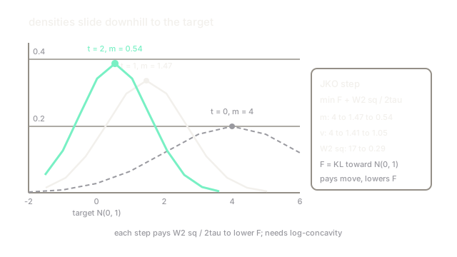
Gaussian through Ornstein-Uhlenbeck flow toward $\mathcal{N}(0,1)$ , start $\rho_0 = \mathcal{N}(4, 4)$ :

Mean: $m_t = 4e^{-t}$ . At $t = 1$ : $1.472$ . At $t = 2$ : $0.541$ .
Variance: $v_t = 1 + 3e^{-2t}$ . At $t = 1$ : $1.406$ . At $t = 2$ : $1.055$ .
$W_2^2$ to target: $m_t^2 + (\sqrt{v_t} - 1)^2$ . At $t=0$ : $16 + 1 = 17$ . At $t=2$ : $0.293 + 0.0007 \approx 0.294$ . Contraction by factor $\approx 58$ in 2 time units, matching exponential decay visibly.

Watch Out For

Discretizing the flow with plain Euclidean steps

Particle updates ignoring the continuity structure leak mass or break positivity. Density histograms go negative and entropy estimates explode.

Use JKO, blob, or kernelized (SVGD) discretizations that preserve the transport structure.

Expecting contraction without log-concavity

Multimodal targets break the exponential rate; flows stagnate between modes exactly like Langevin without mode hops. Theory quotes assuming strong convexity do not transfer.

Check isoperimetry (log-Sobolev) or add tempering for multimodal targets.

The Quick Version

Wasserstein gradient flows descend functionals over distributions, not points.
Velocity fields follow the gradient of the functional's first variation.
JKO steps discretize by trading functional drop against transport cost.
Langevin and Fokker-Planck are the KL-functional special case.
Contraction needs log-concavity; multimodality stalls the flow.