Diffusion Processes

Continuous Markov paths with drift plus noise. Their generators, time scales and stationary laws decide how fast samplers mix and how diffusion models noise data.

Two Langevin paths from opposite starts merge within 2 units and then wander jointly inside the stationary width

Why Does This Exist?

Langevin sampling, diffusion noising and stochastic optimisation all run diffusions $dX = -\nabla V\,dt + \sqrt{2}\,dW$ with potential $V$ shaping the landscape. Practitioners set step counts, noise scales and temperatures by feel. Without mixing theory those choices are blind: too few steps leave bias, too many waste compute, wrong temperature targets the wrong law.

Diffusion process theory gives the dials. The generator encodes local motion, the stationary density is proportional to $\exp(-V)$ , and curvature (convexity of $V$ ) sets exponential contraction rates. Coupling arguments turn curvature into wall-clock mixing times. Stochastic differential equations define the paths; Fokker-Planck tracks their densities; here the focus is long-run behaviour samplers live on.

Prerequisite in one paragraph. You need the Markov property (future depends only on now) and the stationary density $\pi \proportionally \exp(-V)$ . Strong convexity means $V$ curves upward at least quadratically. Background is in Markov chains and Brownian motion.

Think of It Like This

Two leaves in a funnel with shaking

Drop two leaves on opposite rims of a funnel and shake the table. Both slide down, jitter sideways, and soon swirl together at the neck. After merging they move jointly: same region, same spread, past starts forgotten. Steeper funnels merge faster; flat trays never merge.

Diffusions couple the same way. Drift funnels paths together, noise shakes them, and curvature is steepness. The merged law is stationarity; the merge time is mixing.

Where the analogy stops: leaves collide physically while couplings are mathematical joint constructions. Multimodal potentials are multi-funnel trays where crossings take exponential time, which one funnel hides.

How It Actually Works

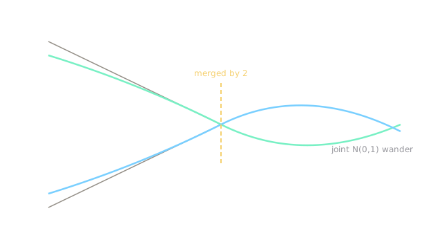
Langevin diffusion $dX = -\nabla V\,dt + \sqrt{2}\,dW$ has stationary $\pi \proportionally e^{-V}$ and generator $Lf = -\nabla V \cdot \nabla f + \Delta f$ giving expected local change. If $V$ is $\alpha$ -strongly convex, two coupled paths with shared noise contract as $E[\lVert X_t - Y_t \rVert^2] \le e^{-2\alpha t}E[\lVert X_0 - Y_0 \rVert^2]$ . Distance halves every $\ln 2/(2\alpha)$ units.

Worked example

Take $V(x) = x^2/2$ so $\alpha = 1.0$ (standard Gaussian target). Starts at $-4$ and $+4$ sit $8$ apart. Contraction gives RMS gap $8e^{-t}$ : at $t = 1$ , $8 \times 0.368 = 2.94$ ; at $t = 2$ , $8 \times 0.135 = 1.08$ , inside the stationary standard deviation $1.0$ . Halving time $\ln 2/2 \approx 0.347$ units, diagram $0.35$ . By $t = 2$ the starts are forgotten and both paths wander in $N(0,1)$ jointly. Discretised Langevin with step $0.01$ needs about $200$ steps to mirror this, the sampler budget the theory predicts.

A double-well $V$ with barrier $8$ instead mixes in about $e^8 \approx 2980$ units: same SDE form, exponentially slower from multimodality.

Watch Out For

Assuming convexity mixing on multimodal targets

The $e^{-2\alpha t}$ rate needs global strong convexity. Mixture targets with separated modes mix by rare barrier crossings, not contraction. Quoting $0.35$ halving on a two-moon posterior promises $200$ -step mixing while true runs need millions.

Fix: check modality first. Multimodal targets need tempering, mode-hopping or exponential-time honesty.

Confusing stationary with converged at finite time

Stationary $\pi$ is the infinite-time limit. At $t = 0.5$ with gap $4.85$ the law is still far from $N(0,1)$ and sampler averages carry transient bias. Reporting them as stationary samples understates error.

Fix: burn past several halving times (here $2$ units) before collecting. Diagnose with coupled gaps, not eyeballed traces.

The Quick Version

Langevin diffusions target $\exp(-V)$ with generator tracking local expected change.
Strong convexity $1.0$ halves coupled distances every $0.35$ units; opposite starts merge by $2$ units.
Discretised runs need about 200 steps of $0.01$ to mirror that mixing.
Multimodal barriers replace contraction with exponential crossing times near $2980$ units at barrier $8$ .
Burn past several halving times before treating draws as stationary.