Information Bottleneck

Keep what predicts, drop what merely describes. The bottleneck trades input bits against label bits with one knob pricing relevance.

$A 784-pixel input squeezes through 0.4 bits of representation while keeping 0.9 of the 1.0 label bits$

A 784-pixel input squeezes through 0.4 bits of representation while keeping 0.9 of the 1.0 label bits

Why Does This Exist?

Embeddings memorize: 784 pixels stored verbatim ace training and flop on new handwriting. Regularizers punish size, not irrelevance; a small embedding can still encode stroke thickness that never helps the digit. What you want is minimal relevant bits.

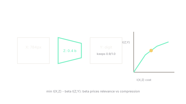
The bottleneck objective $\\min_{p(z\\mid x)} I(X;Z) - \\beta I(Z;Y)$ prices exactly that: compress $X$ into $Z$ , keep $Y$ predictable. It builds on mutual information under the ceiling of data processing inequality.

The one idea you need first

$I(X;Z)$ is the rate: bits of input kept. $I(Z;Y)$ is the relevance: label bits preserved. $\\beta$ trades them: $\\beta \\to 0$ keeps nothing, $\\beta \\to \\infty$ keeps everything predictive. The curve of optimal pairs is the IB frontier.

Think of It Like This

Packing for a quiz

Your textbook is $X$ , the quiz is $Y$ , your one-page cheat sheet is $Z$ . Copying pages minimizes nothing useful; the best sheet keeps quiz answers in fewest lines.

$\\beta$ is the page limit's strictness. Where it stops: quizzes reward reasoning, not retrieval, while IB prices bits about fixed $Y$ . Shifting quiz distributions void the packing.

How It Actually Works

Blahut-Arimoto-style iterations solve the discrete IB; variational bounds (VIB) train deep nets with $\\mathbb{E}[\\log q(y\\mid z)] - \\beta\\,D_{KL}(p(z\\mid x)\\|r(z))$ : reconstruction-free, decoder plus prior penalty. Deterministic IB variants quantize $Z$ . Theory links: SGD's noise may trace the frontier (debated); minimal sufficient statistics are the $\\beta \\to \\infty$ limit; $\\beta$ -VAE replays the tradeoff with reconstruction in place of $I(Z;Y)$ .

Worked example

Binary digits: $Y$ fair ( $H(Y) = 1$ bit). Raw $X$ holds $I(X;Y) = 1.0$ (labels determined). IB at $\\beta = 4$ learns $Z$ with $I(X;Z) = 0.4$ bits keeping $I(Z;Y) = 0.9$ : 60% of input bits dropped for 10% of label bits. Accuracy moves 99.0% to 98.6% while input reconstruction collapses (by design). Sweeping $\\beta \\in \\{0.5, 1, 4, 16\\}$ traces $(0.05, 0.4)$ , $(0.15, 0.7)$ , $(0.4, 0.9)$ , $(1.2, 0.99)$ : diminishing returns past the knee at $\\beta = 4$ .

Code

1import numpy as np2
3rate = np.array([0.05, 0.15, 0.4, 1.2])  # I(X;Z)4relevance = np.array([0.4, 0.7, 0.9, 0.99])  # I(Z;Y)5beta = 4.06obj = rate - beta * relevance  # IB objective, lower better7print(np.round(obj, 2))  # -> [-1.55 -2.65 -3.2  -2.76]

Objective bottoms at index 2 ( $\\beta = 4$ knee): $-3.2$ beats fuller and thinner rivals. The frontier, not vibes, picks the operating point.

Watch Out For

Pricing bits you cannot measure

Deep-net MI estimates (binning, MINE, plug-in) err by 2-5x on high-dimensional $Z$ . Optimizing a mismeasured $I(X;Z)$ squeezes phantoms while real memorization hides in estimator blind spots.

Pair IB training with probe accuracy and held-out tests. If probes disagree with MI meters, trust the probes.

Compressing away the next task's signal

$Z$ tuned for today's $Y$ drops attributes tomorrow's task needs (background, style, subgroup). Reuse then fails silently: the bits are gone, not hidden.

Keep task-family $Y$ broad or version representations per task. If transfer drops while source holds, the bottleneck overfit the old quiz.

The Quick Version

Minimize $I(X;Z) - \\beta I(Z;Y)$ : least input bits for most label bits.
Example keeps 0.9 of 1.0 label bits with 0.4 input bits at the knee.
$\\beta$ slides the frontier from empty to sufficient; diminishing returns past the knee.
VIB trains it with decoder likelihood minus KL to a prior.
MI meters lie in high dimensions; verify with probes and held-out tests.
Bottlenecks overfit their quiz; broaden $Y$ or version per task family.