Math

Mutual Information

How much knowing one variable shrinks your uncertainty about another — which catches every kind of dependence, including the curved and the categorical relationships correlation reports as zero.

Why Does This Exist?

Correlation measures one thing: whether a straight line fits. That is a much narrower question than "are these two variables related", and the gap between them causes real failures.

A feature that determines the label perfectly through a U-shape has a Pearson correlation of zero. A categorical feature has no correlation at all, because there is no line to fit to unordered values. A feature that matters only in one region of its range gets averaged down to nearly nothing. In every case a correlation screen deletes a feature that carries the answer.

Mutual information asks the question you actually meant: how many bits does knowing $Y$ save me when I have to describe $X$ ? No assumption of linearity, no assumption of an ordering, no assumption about the shape of anything.

Three places it appears directly:

Every decision tree split using the entropy criterion is a mutual information calculation. "Information gain" is this quantity, computed between the candidate feature and the label. Understanding its bias — covered below — is what explains why an ID column wins every split.
Contrastive learning objectives are mutual information bounds. InfoNCE, the loss behind SimCLR and CLIP, maximises a lower bound on the mutual information between two views of the same thing. The name is literal.
Clustering evaluation runs on it. When you have no ground-truth labels to score against but two clusterings to compare, Adjusted Mutual Information is the standard measure, precisely because it does not care that cluster IDs are arbitrary.

Think of It Like This

Two overlapping weather reports

You need to know tomorrow's weather in two cities. Each report has some uncertainty: London might be wet or dry, and so might Reading, forty miles away.

If you learn London's forecast, how much have you learned about Reading? A lot — the same weather system crosses both. Not everything, but the uncertainty about Reading has visibly shrunk. That shrinkage, measured in bits, is the mutual information between them.

Now do the same for London and Melbourne. Learning London's forecast tells you nothing about Melbourne. The uncertainty about Melbourne is exactly what it was. Mutual information: zero.

Three things this picture gets exactly right:

It is symmetric. London tells you as much about Reading as Reading does about London. This is the sharp contrast with KL divergence, where the argument order changes the answer. Mutual information is built from KL and is nevertheless symmetric, because the two things it compares — the joint distribution and the product of the marginals — are each symmetric in $X$ and $Y$ .

Zero means genuinely independent. Not "no linear trend" — independent. Nothing about $Y$ helps with $X$ in any way at all.

It says nothing about direction or mechanism. Reading's weather does not cause London's. A shared cause produces the same overlap as a direct one. Mutual information detects that two things move together and is silent on why, which is why it is a screening tool and never an argument for causation.

And one thing the analogy hides, which matters more than any of the above: you never have the true distributions. You have a sample. Estimating this quantity from data introduces a bias that is large, systematic, and points in one direction — always upward. The second pitfall is entirely about that.

How It Actually Works

Start from uncertainty. Entropy $H(X)$ is how uncertain you are about $X$ . Conditional entropy $H(X \mid Y)$ is how uncertain you still are after learning $Y$ . Mutual information is the difference:

I(X; Y) = H(X) - H(X \mid Y)

In plain words: the uncertainty you had, minus the uncertainty you have left. The reduction is the information.

Because $H(X) + H(Y) - H(X, Y)$ gives the same quantity, there is a second and more symmetric form:

I(X; Y) = H(X) + H(Y) - H(X, Y)

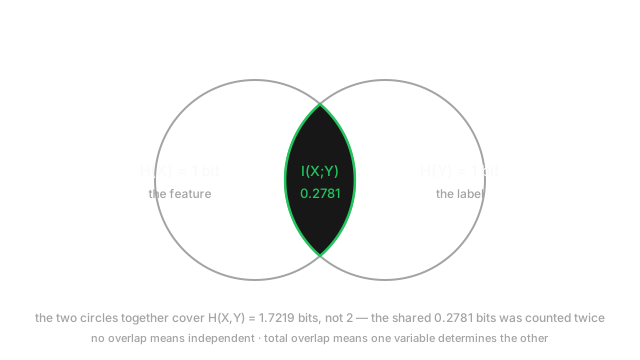
In plain words: add up the two separate uncertainties, subtract the uncertainty of the pair, and what remains is the part you counted twice — the overlap in the diagram above. Written this way the symmetry is obvious: $I(X;Y) = I(Y;X)$ with nothing to prove.

It is a KL divergence

The definition that explains the properties is the third one. Writing $p(x,y)$ for the joint distribution and $p(x)p(y)$ for what the joint would be if the two were independent:

I(X; Y) = D_{\mathrm{KL}}\big(p(x,y) \,\big\|\, p(x)\,p(y)\big) = \sum_{x}\sum_{y} p(x,y) \log \frac{p(x,y)}{p(x)\,p(y)}

In plain words: mutual information is how far the real joint distribution sits from the pretend one where nothing is related.

Everything follows immediately. It is non-negative, because every KL divergence is — knowing something can never increase your uncertainty on average. It is zero exactly when $p(x,y) = p(x)p(y)$ , which is the definition of independence. And the unit is inherited from the log base: bits for base 2, nats for base $e$ .

Where it beats correlation, precisely

The comparison worth internalising:

Covariance and correlation detect linear co-movement. They are computed from products of deviations, so a relationship that curves back on itself cancels to zero.
Mutual information detects any statistical dependence, because it compares whole distributions rather than summarising each one by a mean and a spread.

The cost of that generality is real, and it is why correlation has not been retired: mutual information needs an estimate of the joint distribution. For two continuous variables that means binning, or a nearest-neighbour estimator, and either introduces choices that change the answer. Correlation needs two means and a covariance, computes in one pass, and has a known sampling distribution. Use correlation when a line is a plausible model of the relationship. Use mutual information when it is not, or when you do not know.

Normalising it so the number means something

Raw mutual information is bounded above by $\min(H(X), H(Y))$ , and that bound depends on the variables. A feature with 2 possible values can contribute at most 1 bit; a feature with 1,000 values can contribute nearly 10. Comparing raw values across features with different cardinalities compares the cardinalities as much as the dependence.

The standard fix divides by something with the same units:

\mathrm{NMI}(X; Y) = \frac{I(X; Y)}{\sqrt{H(X)\,H(Y)}}

In plain words: express the overlap as a fraction of the geometric mean of the two uncertainties, giving a number in $[0, 1]$ . The arithmetic-mean denominator $\tfrac{1}{2}(H(X) + H(Y))$ is also common and is what scikit-learn's default computes. Adjusted Mutual Information goes further and subtracts the value expected by chance, which is the version to use when comparing clusterings with different numbers of clusters.

Worked example

Two binary variables — think of $X$ as a feature and $Y$ as a label. The joint distribution, which must sum to 1:

p(x,y): \quad p(0,0) = 0.4,\ \ p(0,1) = 0.1,\ \ p(1,0) = 0.1,\ \ p(1,1) = 0.4

The marginals come from summing each row and column: $p(X{=}0) = 0.4 + 0.1 = 0.5$ , and by symmetry every marginal is $0.5$ . So $H(X) = H(Y) = 1$ bit exactly — each variable on its own is a fair coin.

Joint entropy uses all four cells:

H(X, Y) = -\left(2 \times 0.4 \log_2 0.4 + 2 \times 0.1 \log_2 0.1\right) = 1.0575 + 0.6644 = 1.7219 \text{ bits}

So:

I(X; Y) = 1 + 1 - 1.7219 = 0.2781 \text{ bits}

In plain words: knowing the feature saves you 0.278 of a bit out of the 1 bit of uncertainty in the label — about 28% of it. There is a real relationship and it is far from deterministic.

Check it the other way. Given $Y = 0$ , the conditional distribution of $X$ is $(0.4/0.5,\ 0.1/0.5) = (0.8,\ 0.2)$ , whose entropy is $0.7219$ bits. By symmetry $Y = 1$ gives the same, so $H(X \mid Y) = 0.7219$ , and $I = 1 - 0.7219 = 0.2781$ . The two definitions agree exactly.

Now the case that makes the point. Let $X$ be uniform on $\{-2, -1, 1, 2\}$ and let $Y = X^2$ , so $Y \in \{1, 4\}$ with probability $0.5$ each.

The covariance is $E[XY] - E[X]E[Y]$ . Here $E[X] = 0$ and

E[XY] = \tfrac{1}{4}\big((-2)(4) + (-1)(1) + (1)(1) + (2)(4)\big) = \tfrac{1}{4}(-8 - 1 + 1 + 8) = 0

so the covariance is zero and the correlation is zero. But $Y$ is a deterministic function of $X$ : once you know $X$ there is no uncertainty left, so $H(Y \mid X) = 0$ and

I(X; Y) = H(Y) - H(Y \mid X) = 1 - 0 = 1 \text{ bit}

Correlation says zero; mutual information says one full bit, the maximum possible. A feature-selection step that thresholds on absolute correlation deletes a feature that determines the target. This is not a contrived case — squared terms, absolute values, distances from a centre and periodic effects all behave this way.

Show Me the Code

1import numpy as np2
3
4def mi_bits(joint: np.ndarray) -> float:5    """Mutual information in bits from a joint pmf, shape (rows, cols), summing to 1."""6    outer = joint.sum(1, keepdims=True) @ joint.sum(0, keepdims=True)  # p(x)p(y)7    m = joint > 0                                       # 0 log 0 contributes 0, not nan8    return float(np.sum(joint[m] * np.log2(joint[m] / outer[m])))9
10print(round(mi_bits(np.array([[0.4, 0.1], [0.1, 0.4]])), 4))  # -> 0.278111print(round(mi_bits(np.full((2, 2), 0.25)), 4))               # -> 0.0   independent12
13x = np.array([-2.0, -1.0, 1.0, 2.0])                          # Y = X squared14print(round(float(np.corrcoef(x, x**2)[0, 1]), 4))            # -> 0.0   no correlation15print(mi_bits(np.array([[0, .25], [.25, 0], [.25, 0], [0, .25]])))  # -> 1.0  one full bit16
17rng = np.random.default_rng(0)                                # independent integers18h = np.histogram2d(rng.integers(0, 10, 400), rng.integers(0, 10, 400), bins=10)[0]19print(round(mi_bits(h / 400), 3))                             # -> 0.152  pure noise

The first four prints reproduce the hand calculations exactly. The last one is the warning: two provably independent variables, and the estimate is 0.152 bits rather than 0. Nothing is wrong with the code.

Watch Out For

Comparing raw mutual information across features with different cardinalities

$I(X;Y)$ cannot exceed $\min(H(X), H(Y))$ , and $H(X)$ grows with the number of distinct values $X$ takes. So the ceiling is different for every feature, and a comparison of raw values is partly a comparison of ceilings.

Concretely: a binary feature can contribute at most 1 bit. A postcode with 1,700 distinct values can contribute up to $\log_2 1700 \approx 10.7$ bits. Rank your features by raw mutual information and the high-cardinality ones sort to the top whether or not they carry more signal.

This is the classic decision-tree failure, and it has a name. ID3 split on raw information gain, which meant a unique identifier column — a customer ID, a row number, a timestamp — scored perfectly: it partitions the data into singletons, every leaf is pure, and the gain equals $H(Y)$ . The tree achieves zero training error by memorising the index and generalises not at all. C4.5 introduced gain ratio, which divides the gain by the entropy of the split itself, exactly to cancel the cardinality advantage. Scikit-learn's default is Gini rather than entropy, but the same bias is present and max_features plus min_samples_leaf are what hold it back.

What to do:

Normalise before ranking. Divide by $\sqrt{H(X)H(Y)}$ or by $H(X)$ alone if you want a gain-ratio-style penalty.
Bin continuous features to a fixed number of bins so every feature has the same ceiling.
Treat any feature whose cardinality approaches the row count as an identifier until proven otherwise. High mutual information on such a column is evidence of leakage, not of signal.

Trusting an estimate from a histogram, where the bias is always upward

Plug-in mutual information — count, normalise, apply the formula — is biased high, and the bias does not shrink with more bins. It grows.

The reason is mechanical. With finite samples, the observed joint counts never exactly match the product of the observed marginals, and every deviation, in either direction, adds a positive term to the sum. There is no cancellation, so sampling noise reads as dependence. The leading correction, from Miller and Madow, is

\text{bias} \approx \frac{(|X| - 1)(|Y| - 1)}{2n \ln 2} \text{ bits}

Put the code's numbers in: $|X| = |Y| = 10$ bins, $n = 400$ samples, giving $81 / (800 \times 0.693) = 0.146$ bits. The measured value was 0.152 — the prediction and the observation agree. The bias is not a small correction to the estimate; for independent data it is the estimate.

Three consequences that bite:

A "significant" dependence can be entirely bias. With 100 cells and 400 rows you average 4 observations per cell. Any threshold below about 0.2 bits is measuring your sample size.
Finer binning looks like more signal. Double the bins and the estimate rises, which is the opposite of the usual bias–variance intuition and makes bin count a knob that manufactures results.
Continuous variables have no natural answer. For continuous $X$ and $Y$ with a deterministic relationship, the true mutual information is infinite. Any finite number your code returns is a property of the discretisation, not of the variables.

The fixes, in order of how often they are the right one:

Compare against a permutation baseline. Shuffle $Y$ , recompute, repeat 100 times. Subtract the mean, or better, report your value as a percentile of that null distribution. This costs nothing and handles the bias whatever its source.
Use an adjusted estimator. sklearn.metrics.adjusted_mutual_information does the permutation correction analytically for clusterings.
Use a k-nearest-neighbour estimator for continuous data. The Kraskov (KSG) estimator, exposed as sklearn.feature_selection.mutual_info_regression, avoids binning. It has its own sensitivity to $k$ , so vary it and check the answer is stable.
Get more data per cell. The bias scales as $1/n$ , so ten times the data is ten times less bias, and the rule of thumb is at least five expected observations per cell.

And on contrastive losses: an InfoNCE value is a lower bound on mutual information, and a loose one whose tightness is capped by the batch size. Reporting it as an amount of information is a category error.

The Quick Version

Mutual information is the reduction in uncertainty about one variable from learning another: $I(X;Y) = H(X) - H(X \mid Y)$ .
Equivalently $H(X) + H(Y) - H(X,Y)$ — the overlap between two entropies, which makes the symmetry obvious.
It is the KL divergence between the true joint distribution and the product of the marginals, which is why it is non-negative and why zero means genuine independence.
It detects any dependence. Correlation detects only linear dependence, and reports zero for a perfect quadratic relationship that carries a full bit.
Symmetric, unlike KL divergence. Says nothing about direction or causation.
Bounded by $\min(H(X), H(Y))$ , so raw values favour high-cardinality features. Normalise before ranking, or a unique ID wins every split.
Histogram estimates are biased upward by roughly $(|X|-1)(|Y|-1)/(2n \ln 2)$ bits. More bins means more bias, not more resolution.
Use a permutation baseline, an adjusted estimator, or a k-NN estimator. An InfoNCE loss is a lower bound, not a measurement.