Math

Integrals in Probability

For anything measured on a continuous scale, probability is area rather than height — which is why the chance of hitting an exact value is zero and why so many useful quantities have no formula.

For a continuous variable the height of the curve is not a probability; only the shaded area between two points is, which is why the chance of landing on any exact value is zero

Why Does This Exist?

Three things you use constantly are integrals, and none of them make sense without this page.

norm.cdf is an integral. Every p-value, every confidence interval, every z-score lookup is the area under a bell curve up to some point. There is no algebraic formula for it, which is why that function is a numerical routine and why statistics tables existed for a century.

The denominator in Bayes' theorem is an integral. For continuous parameters, the evidence term $P(D)$ requires integrating over every possible parameter value. That integral is the reason Bayesian methods are computationally hard and the reason MCMC and variational inference exist.

The VAE loss is a workaround for an integral. The quantity a variational autoencoder wants — the probability of the data under the model — requires integrating over the whole latent space. It cannot be done, so the ELBO optimises a lower bound instead. Every explanation of a VAE that starts with the ELBO is starting three steps in; the integral is step one.

Think of It Like This

Asking how much a single point on a map weighs

You have a map of a country shaded by population density — people per square kilometre. Dark regions are cities, pale regions are countryside.

Ask "how many people live in this province" and the map answers: multiply density by area and total it up. Ask "how many people live at these exact coordinates" and the map answers zero — a single point has no area, so however dark the shading, it contains nobody.

That is not a defect of the map. It is what a density means. The shading is people per unit area, not people, and you only get people by multiplying by an area. A very dark point tells you the region around it is crowded, and nothing about the point itself.

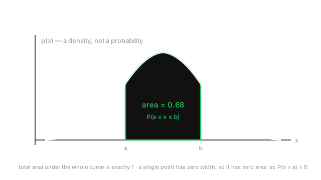
A probability density works identically. Its height is probability per unit of $x$ , not probability. Multiply by a width and you get probability. This is why a density can exceed 1 while a probability cannot — people per square kilometre can be 20,000 without anything being wrong.

How It Actually Works

For a discrete variable, every rule is a sum. For a continuous one, every sum becomes an integral. That is the whole translation, and it is worth seeing all four cases side by side.

Density to probability

A probability density function $p(x)$ satisfies two conditions:

p(x) \ge 0 \quad \text{and} \quad \int_{-\infty}^{\infty} p(x)\, dx = 1

In plain words: never negative, and the total area is exactly one. Probability comes from integrating over an interval:

P(a \le X \le b) = \int_a^b p(x)\, dx

Two consequences follow, and both surprise people:

$P(X = c) = 0$ for any single value $c$ , because an interval of zero width has zero area. This is why continuous variables use $\le$ and $<$ interchangeably — the boundary point contributes nothing.
$p(x)$ can exceed 1. A Gaussian with $\sigma = 0.1$ peaks at about 3.99. Nothing is wrong; it is a rate, not a probability, and the narrowness compensates.

The CDF is the integral of the density

The cumulative distribution function accumulates area from the left:

F(x) = \int_{-\infty}^{x} p(t)\, dt

In plain words: the probability of landing at or below $x$ . It runs from 0 to 1 and never decreases. By the fundamental theorem, differentiating it gives the density back — the CDF and the PDF are an antiderivative pair, which is the most useful single fact on this page.

That relationship is why practical work happens in CDF space. Any interval probability is one subtraction, $F(b) - F(a)$ , and every p-value is a CDF evaluation.

Expectation becomes an integral

The expected value of a discrete variable is $\sum_i x_i P(x_i)$ . Continuous version:

E[X] = \int_{-\infty}^{\infty} x\, p(x)\, dx

In plain words: each value weighted by its density, accumulated across the whole line. Same idea, sum replaced by integral. More generally, $E[g(X)] = \int g(x) p(x)\, dx$ — and this general form is the one that appears everywhere in ML, because a loss is an expectation of a per-example cost.

Variance follows the same substitution: $\text{Var}(X) = \int (x - E[X])^2 p(x)\, dx$ .

The normalising constant, and where things go wrong

Often you can write down a function proportional to a density but not the density itself:

p(x) = \frac{1}{Z} \tilde{p}(x), \qquad Z = \int \tilde{p}(x)\, dx

$Z$ is the normalising constant — the number that forces the total area to 1. In the discrete case it is a sum you can just compute, which is exactly what a softmax denominator is. In the continuous case it is an integral, and that is where tractability dies.

This is precisely the Bayes denominator. Writing $\theta$ for parameters and $D$ for data:

P(\theta \mid D) = \frac{P(D \mid \theta)\, P(\theta)}{\int P(D \mid \theta)\, P(\theta)\, d\theta}

The numerator is easy — likelihood times prior, both of which you chose. The denominator integrates over every possible parameter setting, and for a model with millions of parameters that integral is not merely hard, it is hopeless. Every practical Bayesian method is a way of avoiding it:

Conjugate priors — pick a prior whose algebra makes the integral solvable. Elegant, and only available for a handful of model families.
MAP estimation — maximise the numerator and never compute the denominator, because it does not depend on $\theta$ . This is what regularised training does.
MCMC — draw samples from the posterior without knowing $Z$ . Slow but asymptotically correct.
Variational inference — replace the true posterior with a simpler distribution and optimise a bound. This is the ELBO, and it is what a VAE trains.

Notice that the site's own loss functions are the discrete escape hatch. Cross-entropy works on a categorical distribution where the normaliser is a finite sum over classes, so it is computable. The moment your latent variable is continuous, you are in integral territory.

Worked example

Take the simplest continuous distribution: uniform on $[0, 2]$ . For the total area to be 1 over a width of 2, the density must be constant at $p(x) = 0.5$ .

Probability of landing in the first half:

P(0 \le X \le 1) = \int_0^1 0.5\, dx = 0.5 \times 1 = 0.5

The expected value:

E[X] = \int_0^2 x \cdot 0.5\, dx = 0.5 \left[\frac{x^2}{2}\right]_0^2 = 0.5 \times 2 = 1

In plain words: the average is the midpoint, which is what symmetry demands.

Now a density that exceeds 1. Uniform on $[0, 0.5]$ must have $p(x) = 2$ for its area to be 1. The density is 2, comfortably above 1, and every probability it produces is still at most 1 because the widths are small.

Finally, the Gaussian case. For the standard normal, $P(-1 \le X \le 1) \approx 0.6827$ — the familiar 68% figure, and it is an area. There is no elementary formula for it: $\int e^{-x^2/2} dx$ has no closed form, which is why the diagram above labels that shaded region 0.68 rather than deriving it.

Show Me the Code

1import numpy as np2from scipy import stats3
4
5def uniform_pdf(x: np.ndarray, lo: float, hi: float) -> np.ndarray:6    return np.where((x >= lo) & (x <= hi), 1.0 / (hi - lo), 0.0)7
8
9grid = np.linspace(0, 2, 200_001)                   # fine grid on [0, 2]10pdf = uniform_pdf(grid, 0, 2)                        # constant 0.5, shape (200001,)11print(round(float(np.trapezoid(pdf, grid)), 4))      # -> 1.0    total area12print(round(float(np.trapezoid(grid * pdf, grid)), 4))  # -> 1.0 E[X], the midpoint13
14# A density above 1 is fine: narrow support compensates.15print(uniform_pdf(np.array([0.25]), 0, 0.5)[0])      # -> 2.016
17# The Gaussian has no closed-form integral, so cdf() is a numerical routine.18print(round(stats.norm.cdf(1) - stats.norm.cdf(-1), 4))  # -> 0.6827

Every number matches the hand calculation. np.trapezoid is doing numerical integration — the Riemann idea with trapezoids instead of rectangles — and norm.cdf exists precisely because that particular antiderivative cannot be written down.

Watch Out For

Comparing densities across different units or parameterisations

A density is not invariant under a change of variable, and this trips up model comparison in a way that is genuinely hard to spot.

Rescale $x$ — metres to centimetres, or apply any invertible transform — and the density changes by a Jacobian factor, because the widths you are multiplying by changed. The probabilities are identical; the density values are not. So a log-likelihood of $-2.3$ on one parameterisation and $-4.1$ on another may describe exactly the same model fitting exactly the same data equally well.

The consequences are concrete. Continuous log-likelihoods, and therefore bits-per-dimension figures, are only comparable across models trained on identically preprocessed data. Change your normalisation, your image scaling, or your tokenisation and the numbers shift for reasons that have nothing to do with model quality. Comparing a published bits-per-dimension against your own without matching the preprocessing exactly compares nothing.

Also: a continuous log-likelihood can be positive, since a density above 1 has a positive log. That is not a bug and it is not a probability greater than one.

Assuming a normalising constant can be computed

The most common way a from-scratch probabilistic model fails is that someone writes down an unnormalised density, gets a working loss, and never notices $Z$ was ignored.

Sometimes ignoring it is correct — in MAP estimation and in ordinary regularised training, $Z$ does not depend on the parameters, so it vanishes under optimisation. That is why cross-entropy plus weight decay works without anyone thinking about integrals.

It stops being correct the moment you need an actual probability rather than a ranking. Comparing two models by likelihood, reporting a calibrated confidence, computing an ELBO, or evaluating an energy-based model all require the normaliser, and for continuous latent variables it is an integral over the whole space. Energy-based models are the sharpest case: the energy is easy and $Z$ is intractable, which is the entire reason they are trained with contrastive methods rather than by maximum likelihood.

The practical rule: know whether your objective needs $Z$ . If you are ranking or optimising parameters, you can usually drop it. If you are quoting a number that claims to be a probability, you cannot, and you should say which approximation produced it.

The Quick Version

For continuous variables every probability rule becomes an integral instead of a sum.
A density is probability per unit, not probability. It may exceed 1.
$P(X = c) = 0$ always, because a zero-width interval has zero area.
The CDF is the integral of the density; differentiating the CDF returns the density. They are an antiderivative pair.
Expectation is $\int x\, p(x)\, dx$ , and more usefully $E[g(X)] = \int g(x) p(x)\, dx$ — every loss is one of these.
The normalising constant $Z$ forces the total area to 1. Discrete: a sum, like a softmax denominator. Continuous: often an intractable integral.
Bayes' denominator is that integral, which is why conjugate priors, MAP, MCMC and variational inference all exist.
Densities are not invariant under reparameterisation, so continuous log-likelihoods only compare across identical preprocessing.